In this post we'll have a closer look at Nat Sarkissian's generative FxHash token Eucalyptus and Sagebrush. The token was released on January 12th as a part of the Cure3 exhibition:
Once again, my mind is back in the hills. It's been surprising to discover how much they've influenced me. I'm excited to release "Eucalyptus and Sagebrush" this Thursday as part of the Cure3 event. pic.twitter.com/l3okAJOkCd
— Nat Sarkissian (@_NatSarkissian) January 9, 2023
This post is complementary to Raph's twitch livestream on the 24th of March 2023, where we go over the token in depth:
So many @fx_hash_ masterpieces deserve a closer look! Join @gorillasu and @sableraph live on Twitch tomorrow for an Insider's guide to generative art and creative code.
— Raphaël de Courville (he/him) 𓅬 (@sableRaph) March 23, 2023
In this episode of fx(review) we will explore the Art & Code of 'Eucalyptus and Sagebrush' by @_NatSarkissian pic.twitter.com/vjUCxGlhCo
You can watch the VOD here as well as on Raph's Youtube sometime in the future!
Generative Landscapes
Generative landscape sketches have become one of the most popular type of generative art over the course of the past two years, especially in the context of blockchain art. In part, this surge of popularity can be attributed to the work of artists like Zancan, who has seen great success in that regard.
Zancan's Garden Monoliths, for instance, now stands as the token with the all time highest cumulative transaction volume on FxHash, having aggregated over a million Tezos in secondary sales.
Garden, Monoliths #16 and #19 Respectively
On the flip-side, more and more budding generative artists are attempting this style for themself, simply because a lot of algorithms have been devised for the purpose of creating natural scenes. Many noise algorithms and random number generators can be effectively utilized for the simulation of terrain formation as well as the positioning of wilderness, vegetation and plant growth.
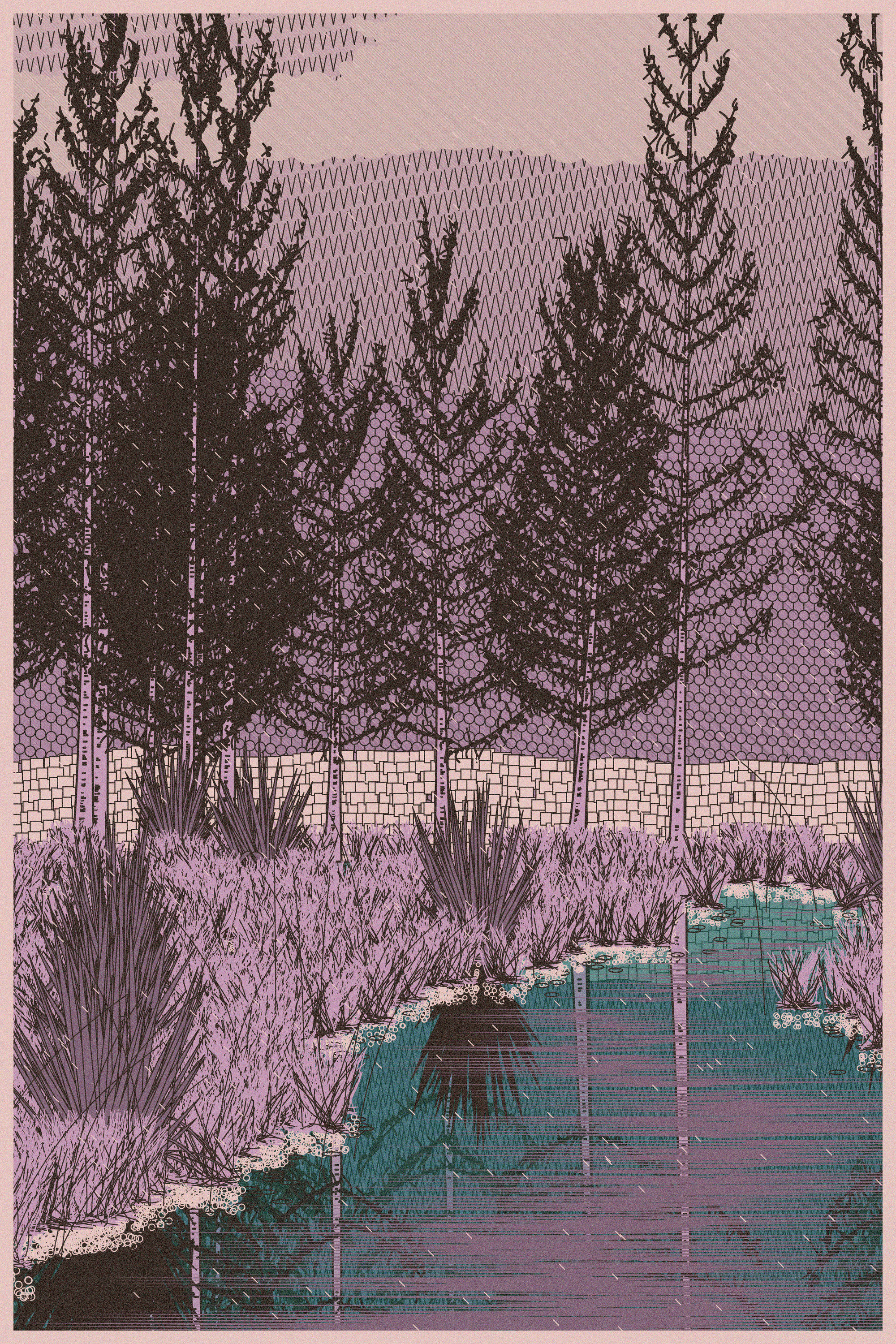
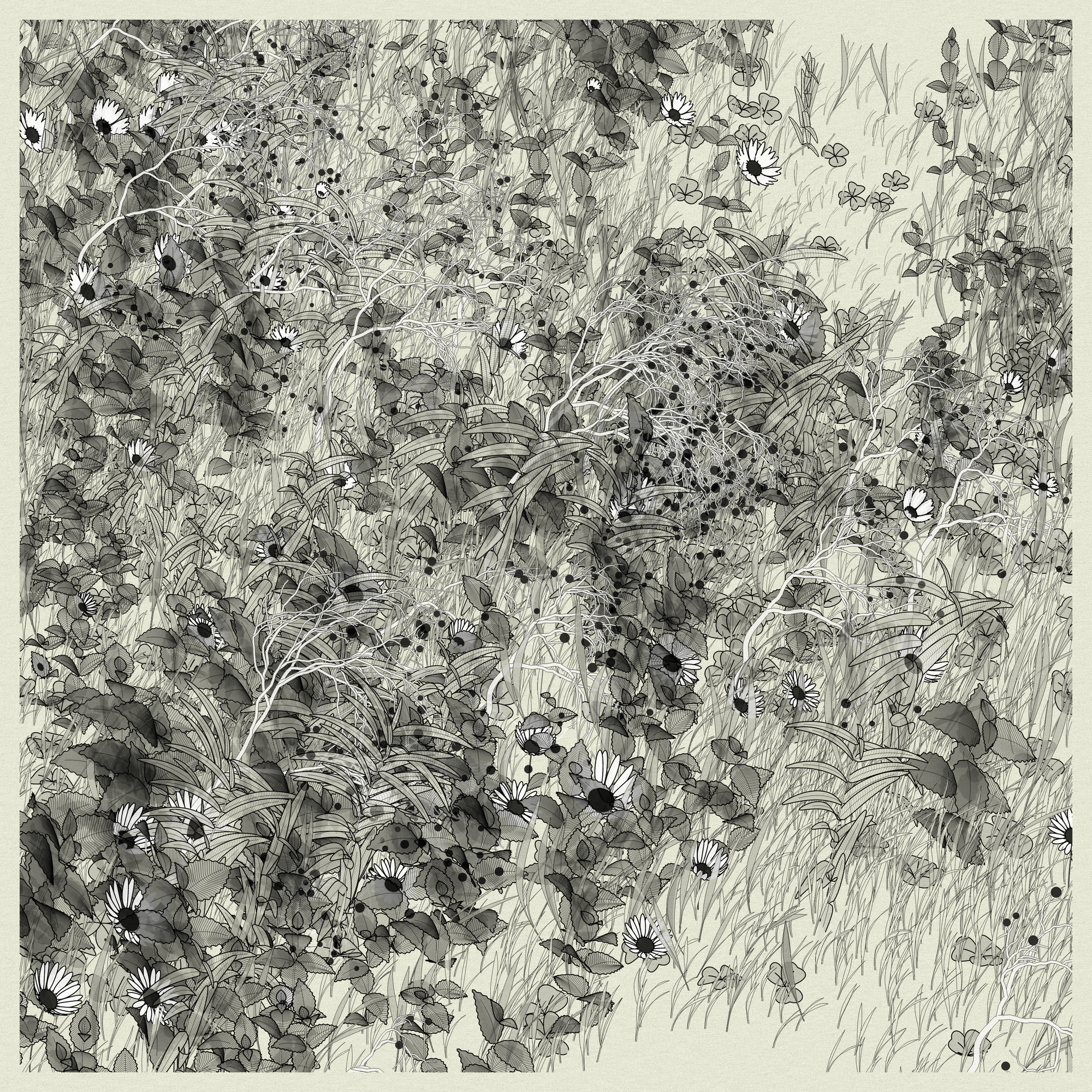
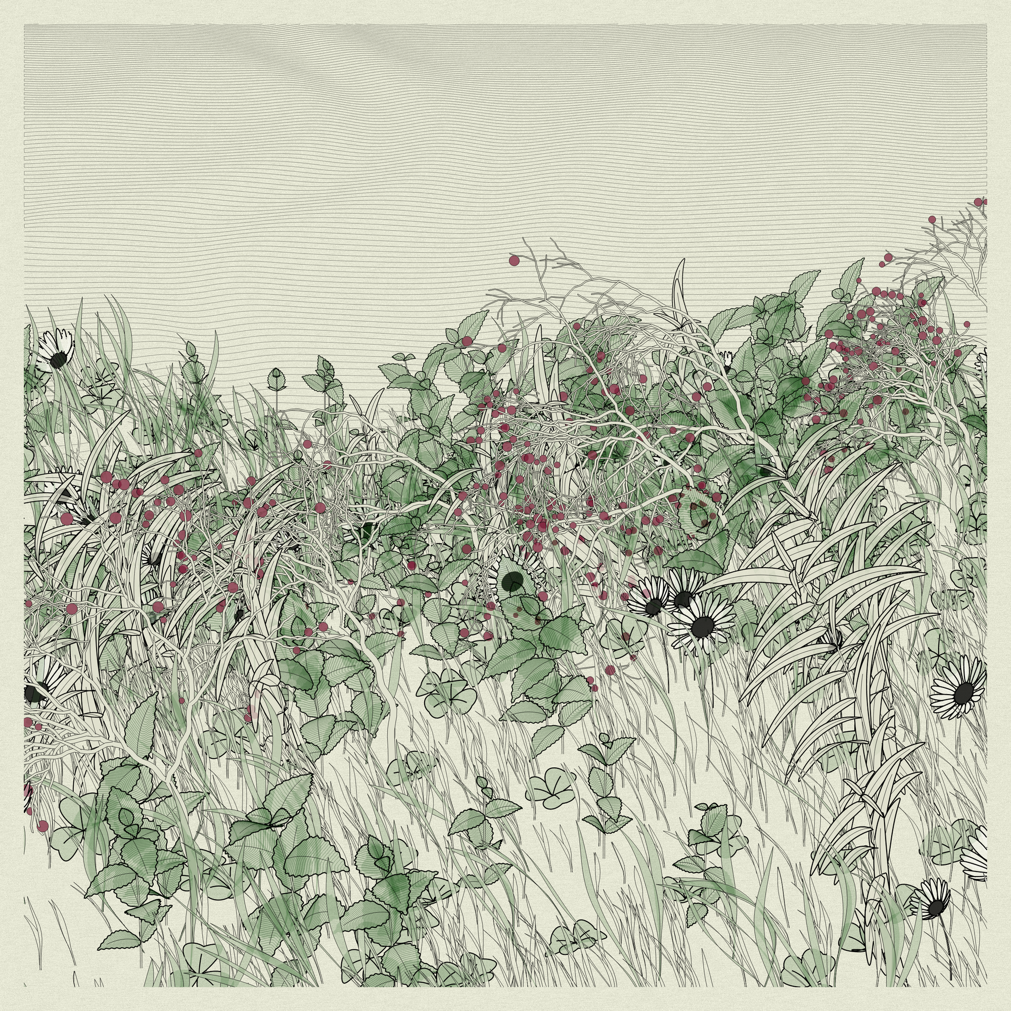
I've attempted landscape sketches myself in the past. I haven't done one for fxhash (yet - but it's coming - probably). I did a sketch back in August 2022 where I tried to simulate grass simply by drawing many short lines to the canvas, where the lines towards the bottom of the canvas are slightly larger and longer, to convey an illusion of distance and depth. Later I also had a pebbly river flow through this landscape:
Smol blobs instead of circles, I think it sells the idea of pebbles a bit more 🤔 #p5js #craetivecoding pic.twitter.com/YzTUXZSw0j
— Ahmad Moussa || Gorilla Sun (@gorillasu) August 21, 2022
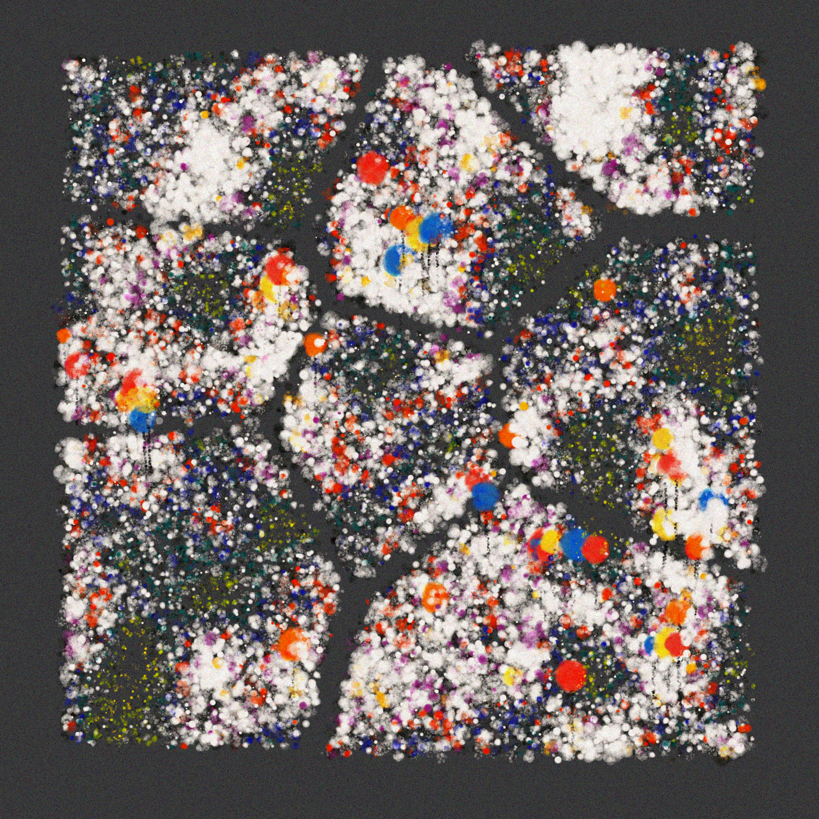
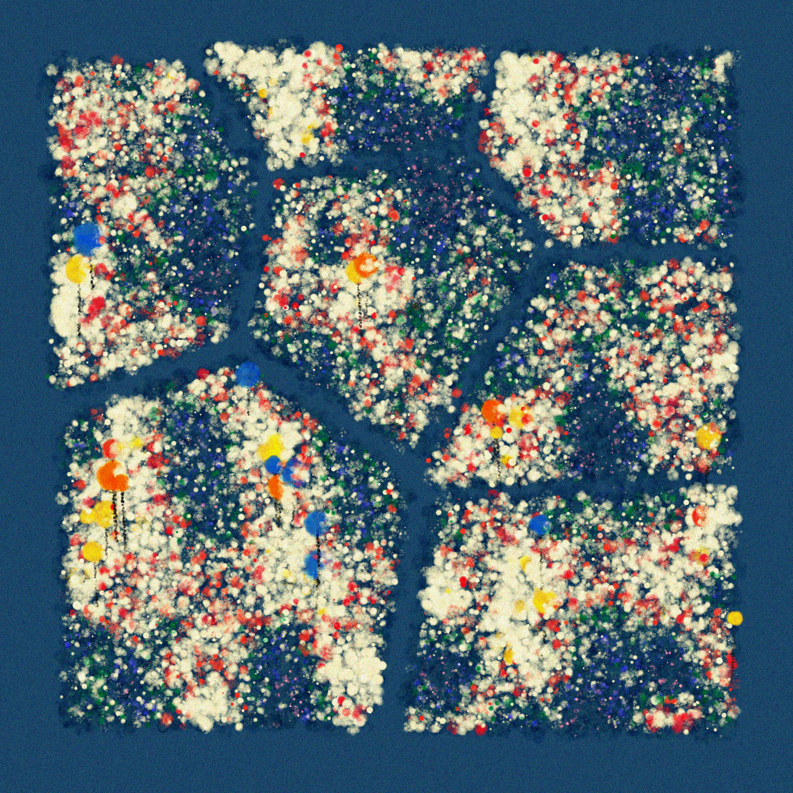
I never returned to this particular project however. Another one that I did recently during Genuary 2023, wasn't initially intended to be a landscape piece, but it reminded me of a mossy meadow, hence I tried to lean into it a little bit more:
Voronoiscapes
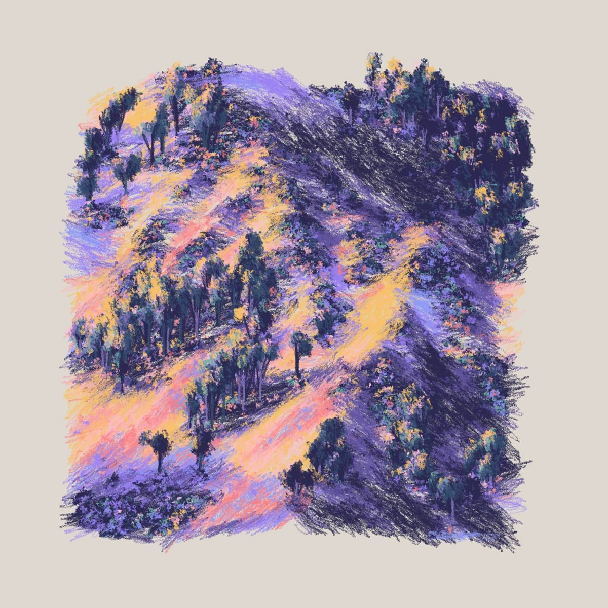
Eucalyptus and Sagebrush
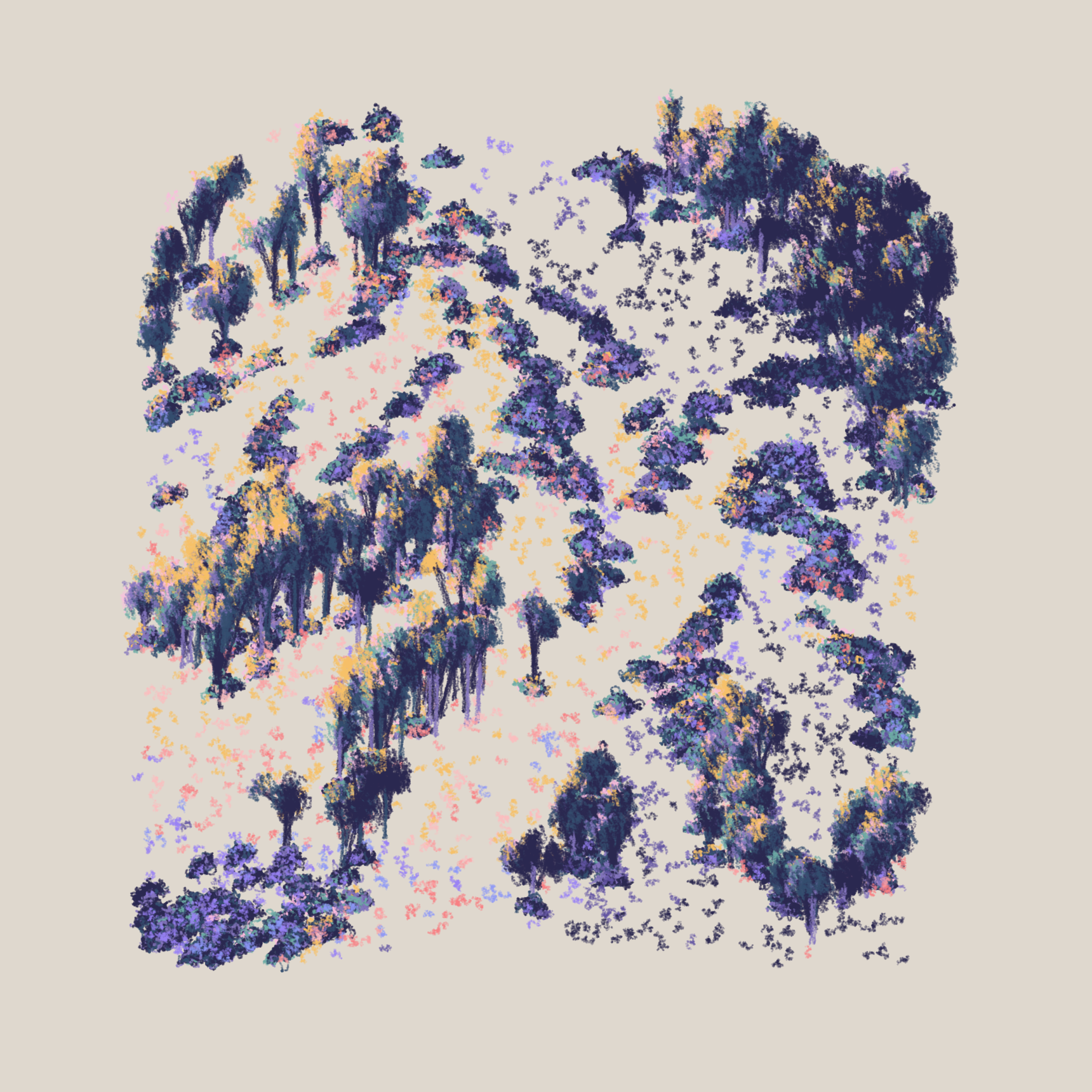
With Eucalyptus and Sagebrush, Nat Sarkissian puts his own spin on the genre:
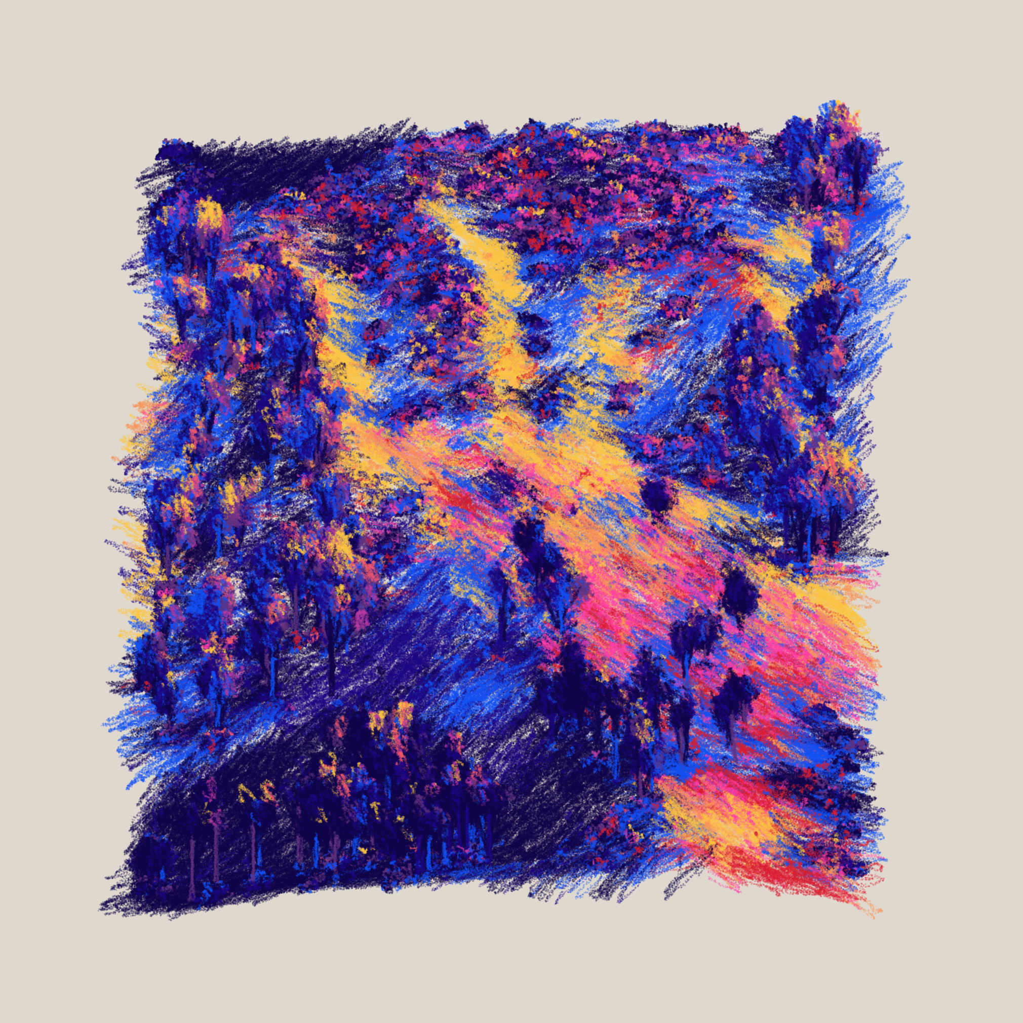
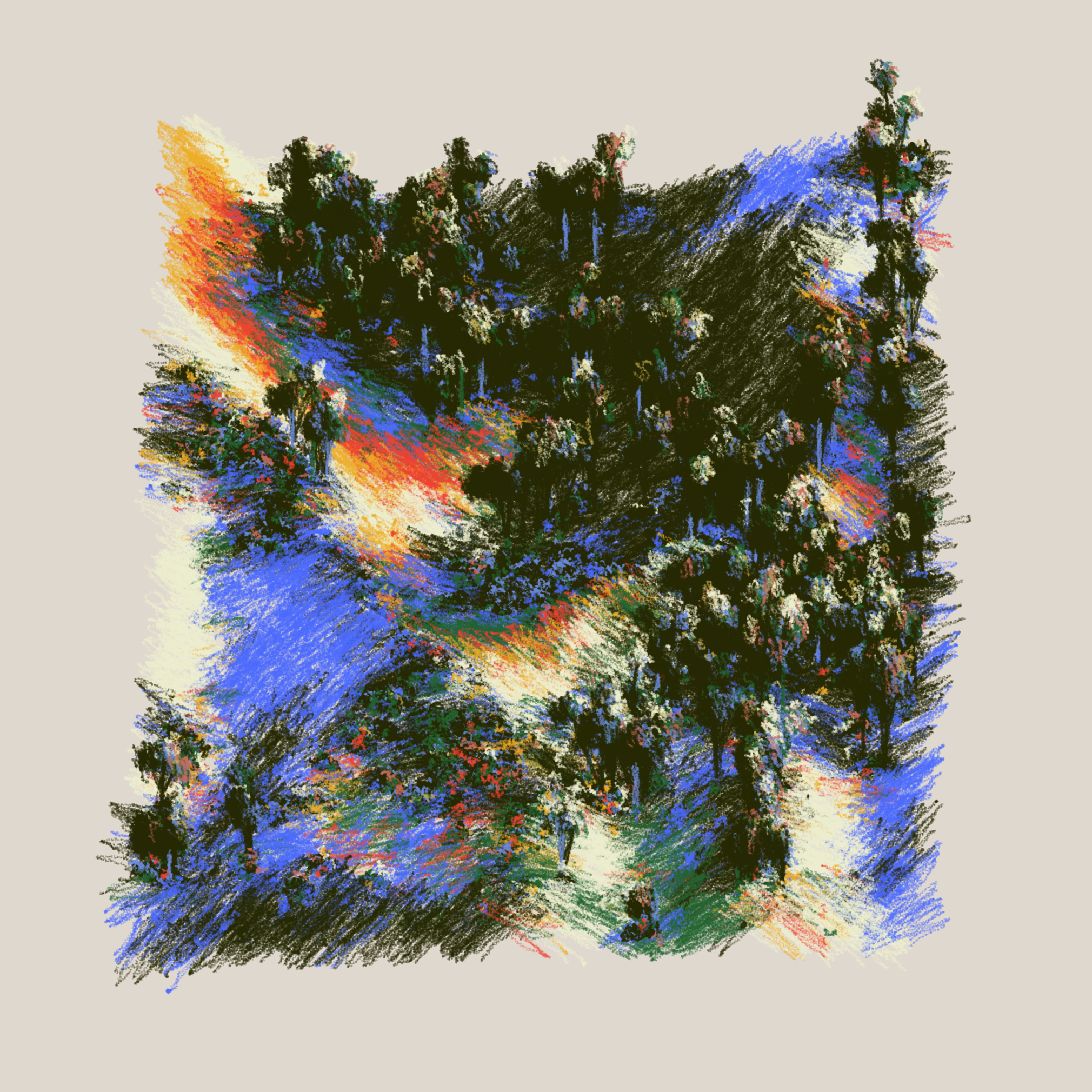
Eucalyptus and Sagebrush #1 and #8
My immediate thought after seeing the artwork for the first time was: 'How? How do you make something generative look so natural?'
The delicate generative brushwork and the interplay between colors - that results in an intricate shading of the terrain - is reminiscent of an impressionist style from an era long past. In impressionism the goal is not to recreate the scene as it exists in reality, but rather, the artist attempts to capture an impression of the subject. Nat says in the token's description:
Each iteration of this algorithm feels, to me, like a glimpse out of a car window on a drive up the coast, a pause on a cool morning hike, or a memory of tearing through sharp underbrush with good company.
In impressionism there is a great focus on lighting and how the illumination interacts with the scene. Often this occurs in combination with delicate and fine brushstrokes, where the coloring of these strokes tries to emulate the incidence of light with different surfaces. Claude Monet is arguably the most acclaimed artist to grace this artistic style:
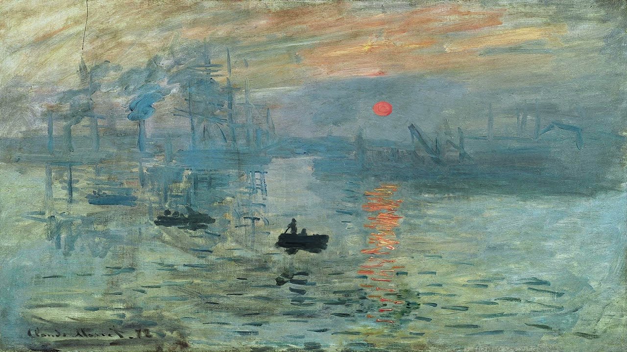
Impression, Sunrise by Claude Monet
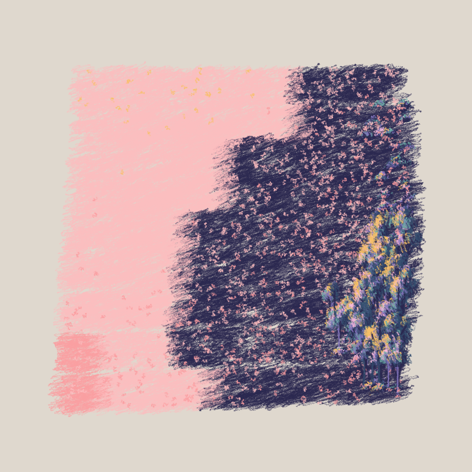
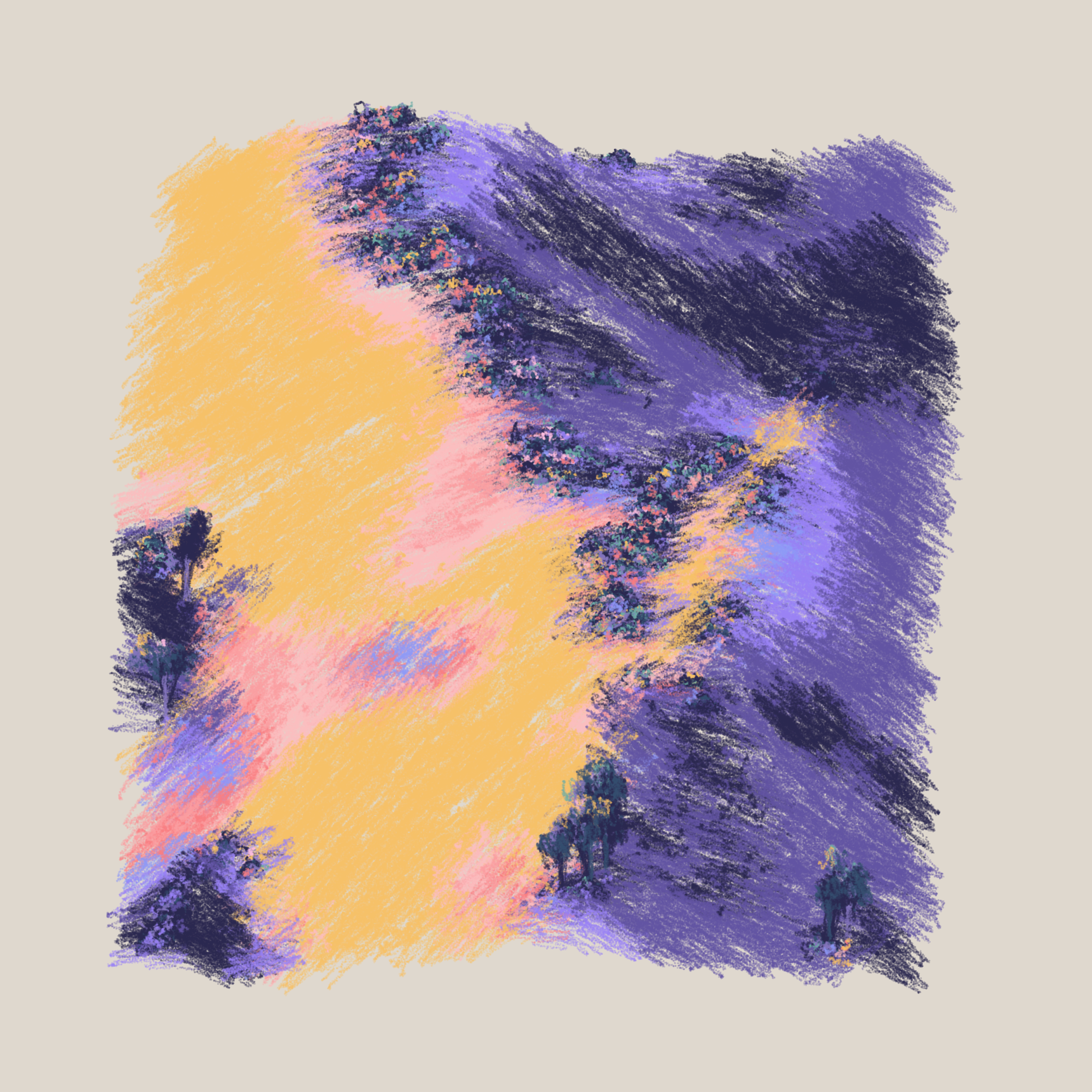
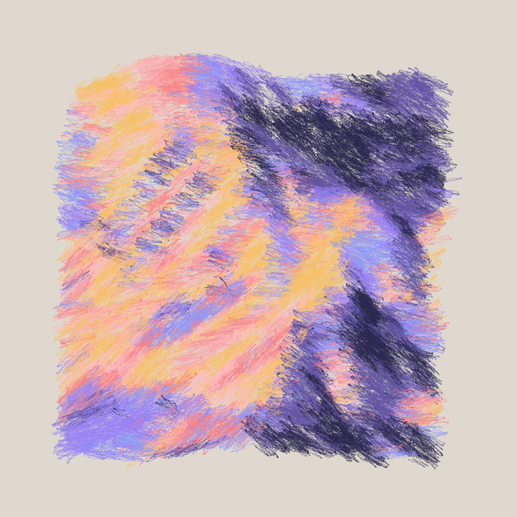
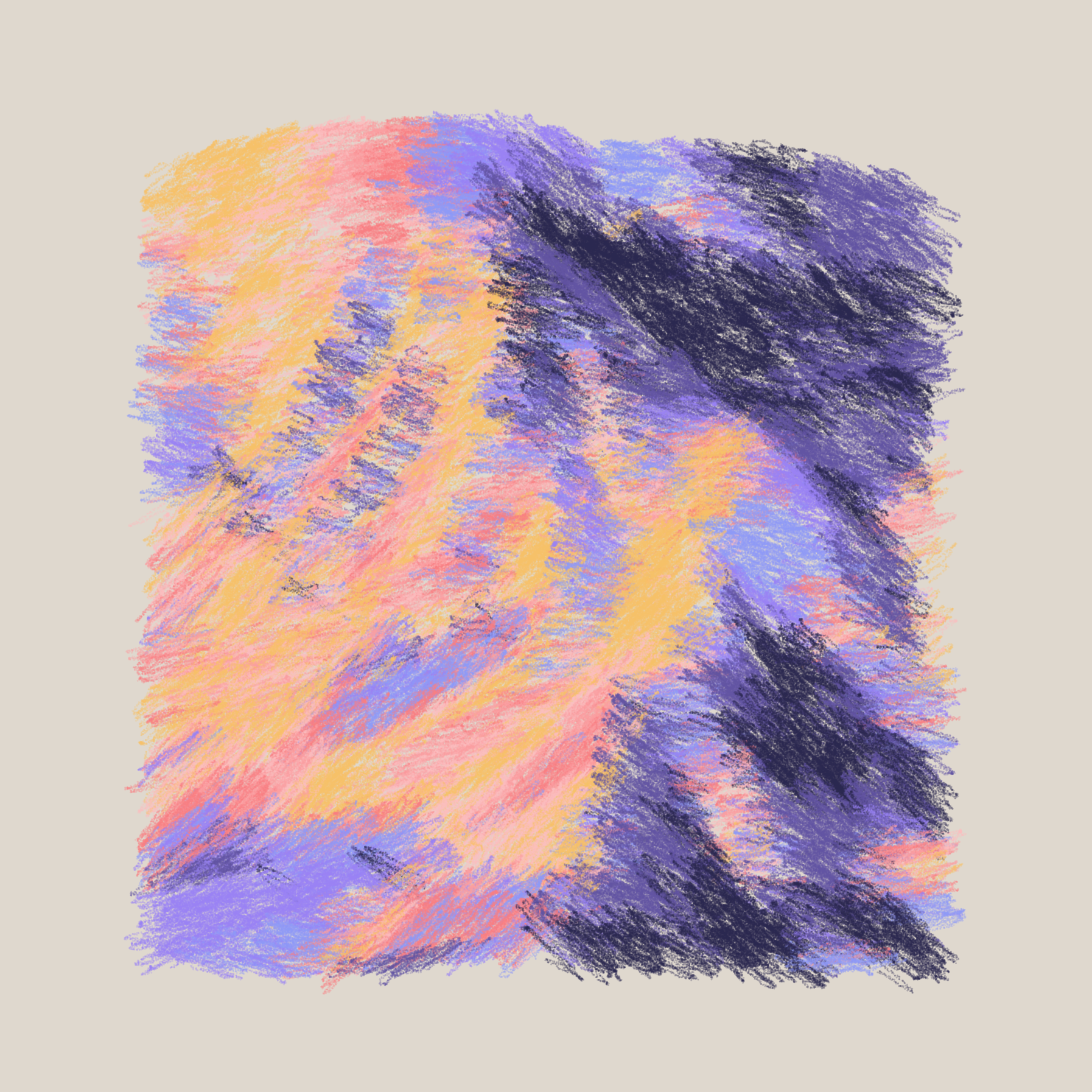
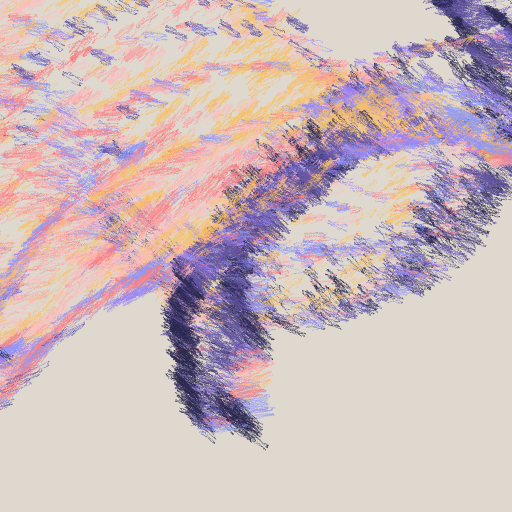
A focus on light, brushwork and coloring can also be seen in Nat's work, especially when we look at it from a distance:
Stylistically and texturally, I drew from landscapes rendered in oil pastels, placing thousands of tiny circles, alluding to the effect of depositing particles of color onto paper.
In Eucalyptus and Sagebrush, what I can't really put my finger is how the terrain is generated, and subsequently how the brushstrokes are placed and colored to create an illusion of shading. It looks very natural, especially when you look at it from a distance. Perlin noise by itself gives you very lumpy shapes, which can work in the right setting, but terrain is usually a bit more shapely, jagged and pointy. Another thing that is a mystery to me is how the illumination works. How are the tips of the trees colored differently, and only from the direction of the light-source? That's what I'm hoping to have figured out by the end of this article.
Hence, the aim of this post is to analyse what goes on behind the scenes in Eucalyptus and Sagebrush, and how the different components of the code work together to create such lush and natural sceneries.
Height Maps
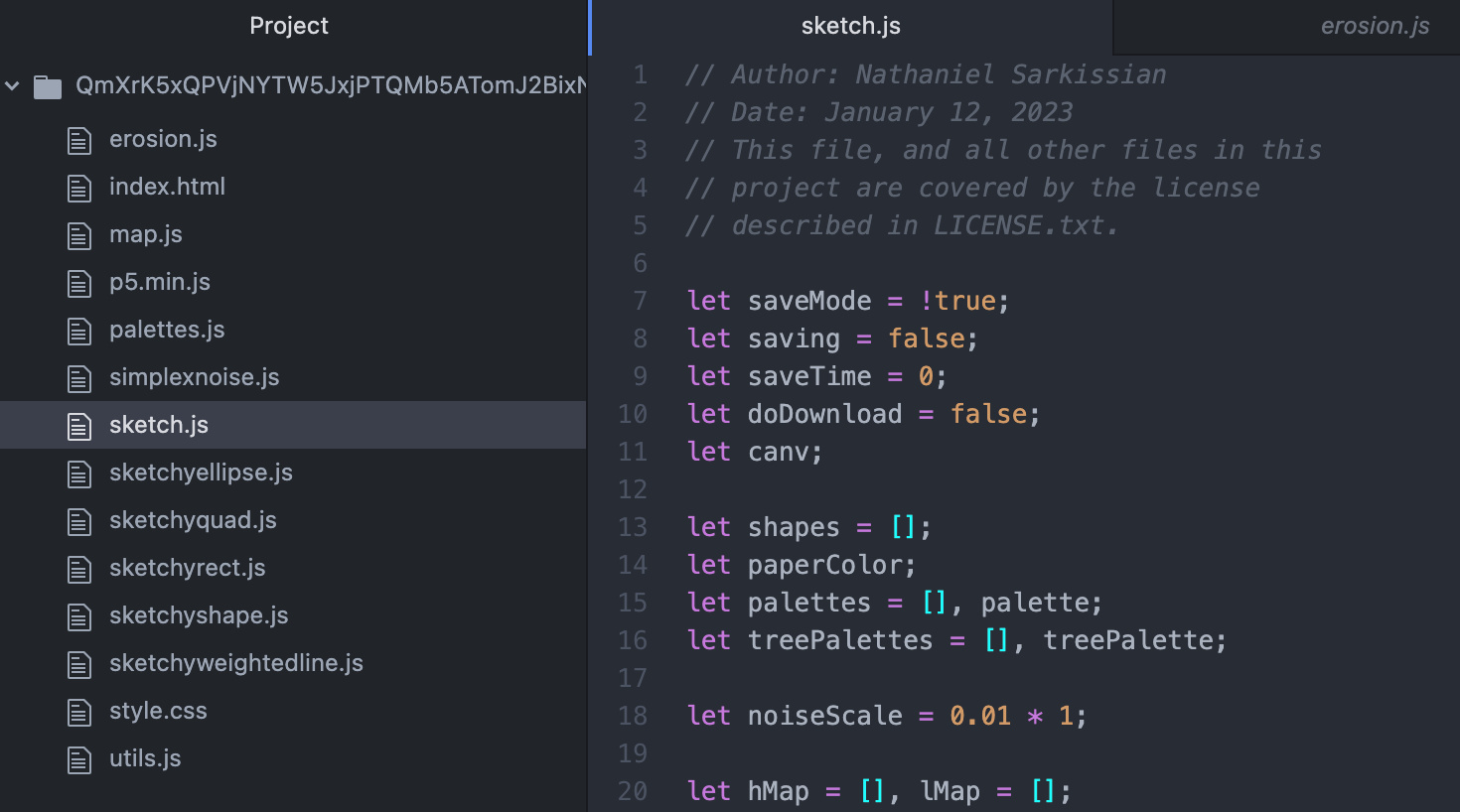
I had a gander at the code and to my surprise found an extremely tidy and readable project. To make things a bit more approachable, and to be able to understand what the variables and parameters in the code do, it was important for me to be able to run the sketch offline. I obtained a local copy of the code with the wget command line tool. For most examples throughout the text, we'll lock in the same seed that is used for the token's preview on fxhash, except when noted otherwise. This makes it easier to see the effects of variable changes as we go over the code.
Nat's project is based on the popular P5 library, making use of it's convenient functions to process values and draw the graphics to a canvas element. Usually, a natural starting point for figuring out projects like this is the sketch.js file, where the centerpiece is the setup() function that ties the entire project together.
The first couple of lines are pretty standard, after initializing a bunch of hyper-parameters, we enter the setup function where we set the fxhash randomness seeds, and create the canvas as well as the graphics buffer, which I assume is in place for responsive resizing purposes of the browser window.
The first two lines for which we'll have to do some digging are:
setupHeightMap()
setupLightMap()
I have a vague idea what height maps are, but haven't really used them before (on purpose at least). I also can't immediately tell how it ties into the narrative of the sketch, when my initial assumption was that the colourful strokes that make the graphic are positioned with some form of perlin noise generated map. But it turns out that Nat is actually using something much more elaborate than that.
Both of the setupHeightMap() and setupLightMap() functions can be found in the map.js file. I did a little bit of research to figure out what heightMaps are generally used for and how they can be created, and we'll go into more detail in the next section, but essentially, height maps serve the purpose of terrain generation, where they specify the elevation of the terrain at any given point. Height maps can then be further shaped into more convincing landscapes by passing them through subsequent algorithms (more on that in the next section as well).
But first things first, how do we create a height map? And what data structure can be used to represent such a height map? To answer the latter, a height map can simply be defined as a 2-dimensional array of numerical values, where the entry of each cell symbolizes the elevation at the given coordinate, where the coordinate is the x and y indices of the array entry.
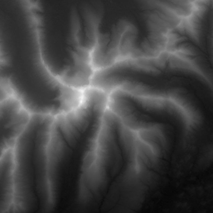
Large scale and small scale heightmap.
As for the creation process, a good introduction to the topic is this fantastic resource by none other than redblobgames, who has written extensively about algorithms for game development. I highly recommend checking out all of his writings.
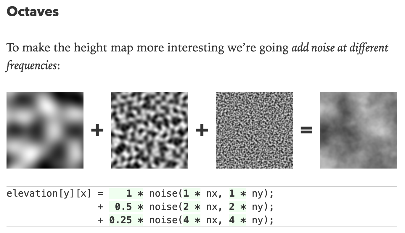
Theoretically, we could just generate a 2D array of random values with Perlin Noise or Simplex Noise, and use those as a starting point for our terrain, for a better foundation though, we usually combine multiple noise maps at different frequencies, which is exactly what the prepareHeightMap() function does.
Let's have a look at the code! The prepareHeightMap() function can be found as the first function within the map.js file.
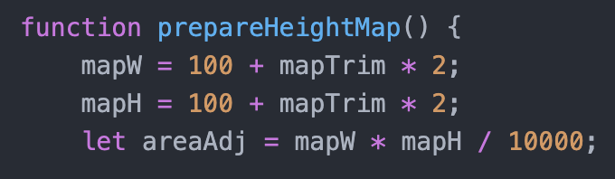
To begin, the parameters mapW and mapH, as they suggest indicate the size of the heightMap and they're both fixed to a value of 100. The size of the heightMap has actually no influence on the number of strokes drawn (we'll see later that that's a separate variable), but rather on how much of a noise field the resulting terrain will span. If we set these parameters to something small, then we're only sampling from a very small range of noise values. Here's what this would look like:
mapW=2, mapH=2 | mapW=10, mapH=10 respectively
In this case no noticeable elevation is generated, but I actually find these minimal ones quite charming as well.
Next up, Nat initializes some random variables that will define the frequency and intensity of three different noise distributions:
let mapScale = random(0.15, 1);
let sustain = map(mapScale, 0.15, 1, 0.6, 0.2);
let noiseDist = [
	[1, 1 * mapScale],
	[sustain, 2 * mapScale],
	[pow(sustain, 2), 4 * mapScale]
];
We're not actually going to create these noise distributions individually, nor store them in arrays. We'll simply loop over the dimensions of the grid and use the parameters we just initialized to sample from these distributions and aggregate the resulting numbers to obtain our height map.
This nested loop, stripped down to the bare minimum, looks as follows:
for (let i = 0; i < mapW; i++) {
  for (let j = 0; j < mapH; j++) {
    let nx = 0;
	  for (let k = 0; k < noiseDist.length; k++) {
	    nx += norm(
            sNoise.noise2D(
              i * noiseScale * noiseDist[k][1] * 2,
              j * noiseScale * noiseDist[k][1] * 2
            ), -1, 1) * noiseDist[k][0];
	  }

    let ns = constrain(pow(map(nx, 0, noiseTotal, 0, 1) * 1, 1), 0, 1);
  }
}
For those who aren't familiar with Simplex noise, it is essentially a better and improved version of Perlin noise. It doesn't come out of the box with P5, but Nat included it in a script file.
As for the norm() function that processes the sampled Simplex noise values, it's also a P5 function and works in a similar fashion to the map() function, which you might be more familiar with. The norm() function always maps from the specified range (2nd and 3rd parameter) to a [0, 1] range. Since the sum of these sampled values can exceed the upper bound of that range, we need to additionally map it to a [0, 1] range in a subsequent step based on the total.
let noiseTotal = 0;
for (let i = 0; i < noiseDist.length; i++) {
  noiseTotal += noiseDist[i][0];
}
And in this manner we've created the height map and could technically store it in an array for later use. There's however a couple more lines within this nested loop that process the values of our height map. Instead of going over each line by itself I'll add comments to the code to explain what they do:
// clamps the number of values behind the decimal point
ns = floor(ns * 100000)/100000;

// maps the height map value to an angle in the range [TAU, 2 * TAU]
ns *= TAU * 2 * map(j, 0, mapH, 1, 0.5);

// we find the highest and lowest point in the height map and store them
let y = map(j, 0, mapH-1, 0, targetSz);
y += map(ns, 0, 2 * TAU, 0, 1) * terrainHt;
if (y < minY) { minY = y; }
if (y > maxY) { maxY = y; }

// finally store the heightmap value
row.push( ns );

// since we are already in a nested loop we can do some other stuff
// like allocating values for an erosion and deposition map
// which will be used in the erosion algorithm of the next section.
let erodeAmt = 0.1;
let depositAmt = 0.001;
erodeMapRow.push(erodeAmt);
depositMapRow.push(depositAmt);
Now that we've created our height map, we can move on to turning it into a shapely terrain with an algorithm that is better known as Hydraulic Erosion!
Terrain Generation and Hydraulic Erosion
Terrain generation is a well researched topic in computer graphics, for which a whole slew of algorithms has been devised. One field of application where it predominantly occurs is in graphics for video games. Some examples are age of empires (2 is one of my favorite childhood games), skyrim as well as the civilzation series. All of which have pretty convincing terrains.
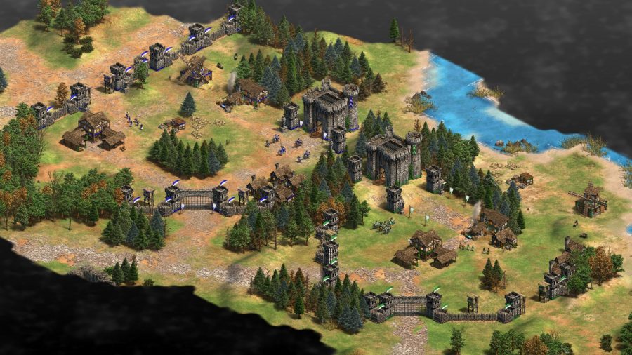
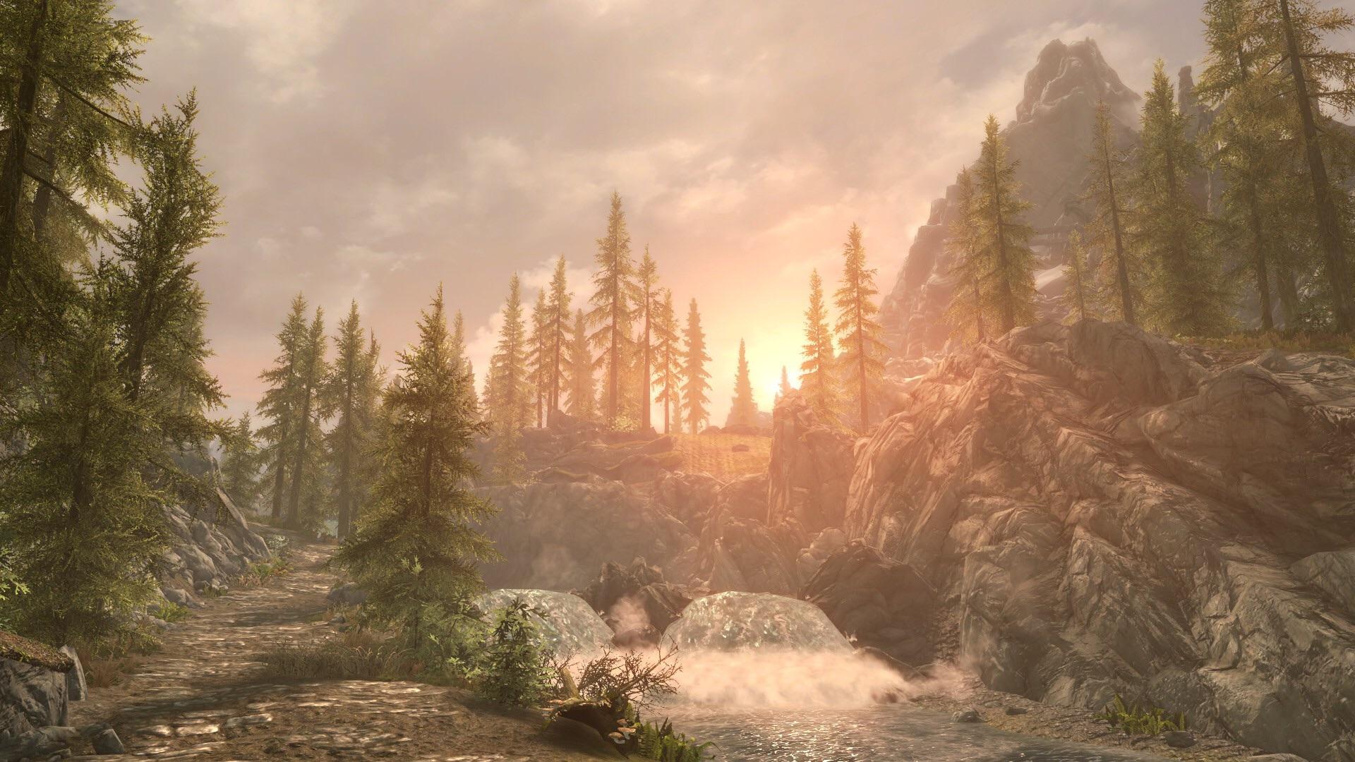
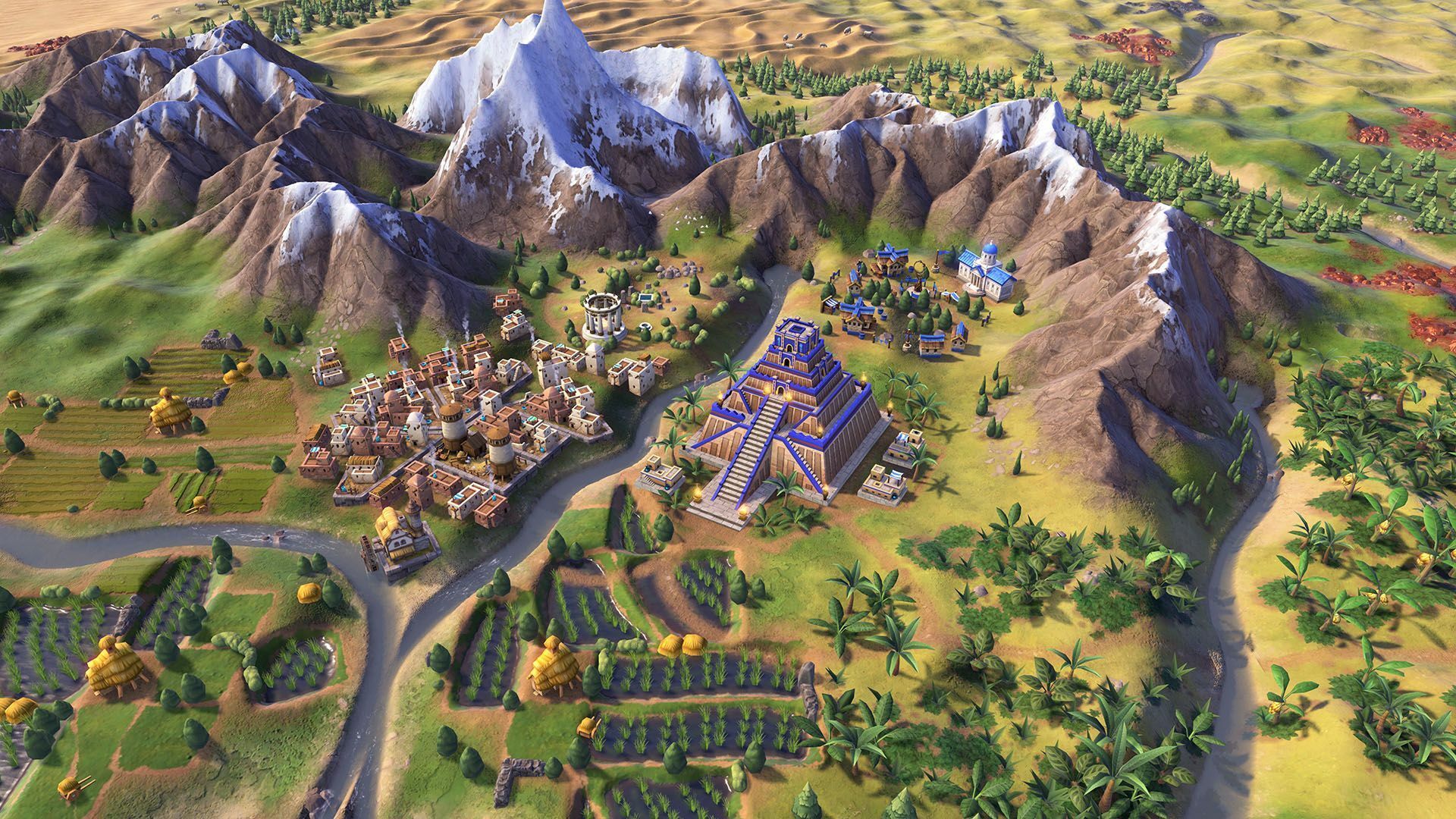
Age of Empires 2 | The Elder Scrolls 5: Skyrim | Sid Meier's Civilization 6
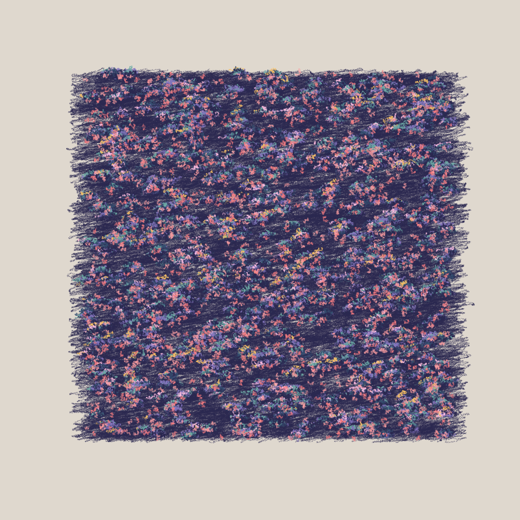
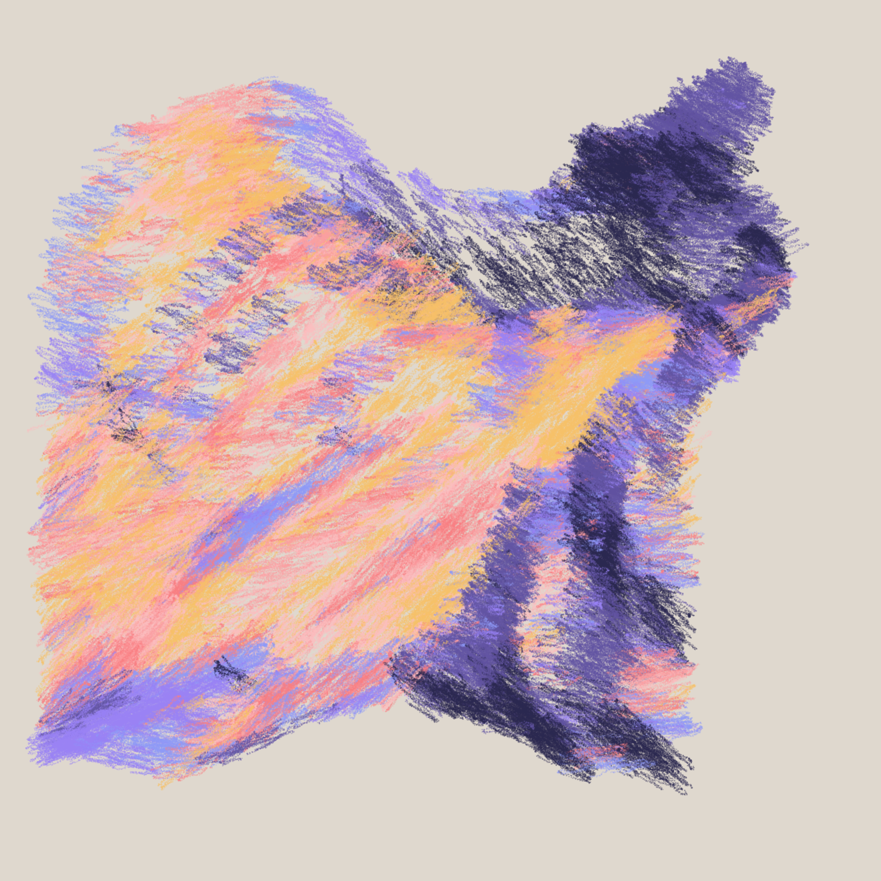
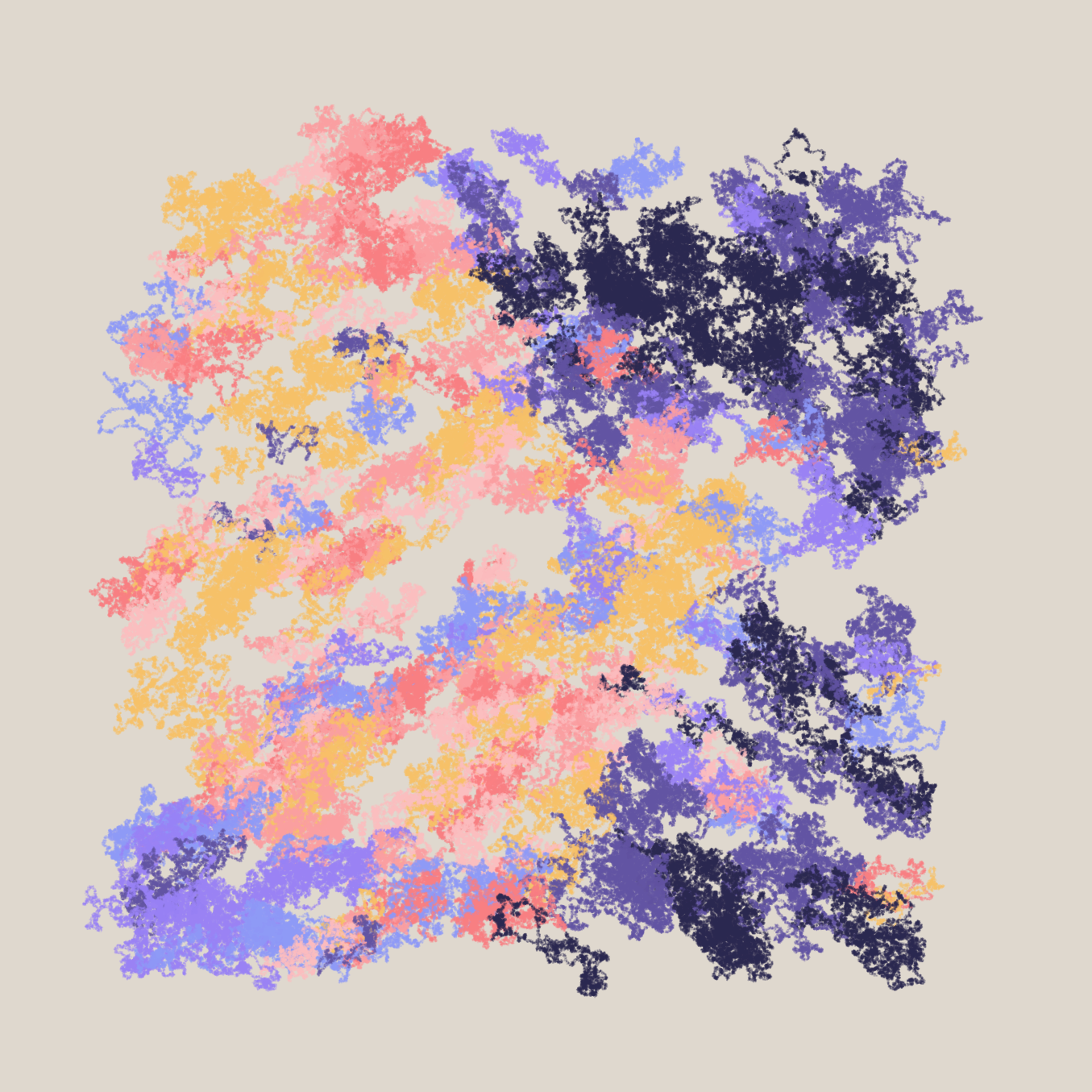
Here's what Eucalyptus and Sagebrush would look like with the terrain shaping algorithm toggled off:
The generated landscape in this case is much duller, flatter, and the ridges aren't as pronounced as they were before. The terrain overall isn't as shapely. So, what's going on in this terrain shaping algorithm? And how does the height map we just created tie into this?
To be more specific the particular algorithm that Nat used is called Hydraulic Erosion. At the very end of the prepareHeightMap() function we found a couple of lines that looks as follows:
erode(hMap, 10000 * areaAdj, 1, 4);
erode(hMap, 10000 * areaAdj, 1, 4);
erode(hMap, 10000 * areaAdj, 1, 4);
erode(hMap, 10000 * areaAdj, 1, 2);
blurMap(hMap, 1, 0.2);
This means that the height map is being passed to this erode() function several times as well as a blurring function apparently. We can find this function in the erosion.js file. A larger comment sits at the top of this file, where Nat mentions that his implementation finds its beginnings with Sebastian Lague's Unity/C# code:
Hydraulic erosion is a relatively well known idea in terrain generation. This implementation started with Sebastian Lague's Unity/C# implementation. Other than porting it to JavaScript and adapting it to the data structures I had in place for this project, I modified somewhat significantly. I removed the erosion brush concept. I modified the scale of a few of the parameters such as sediment capacity, erosion speed, deposit speed, etc. I added functionality to carry the color of the sediment in the rain drops in order to cause the terrain to be colored by the erosion effect.
Comments like this fill my heart with excitement. For one, we're one step closer to figuring out what's happening in the sketch, and additionally we've already learned a little bit about a new algorithm. Now Nat has got me curious: what's this erosion brush concept? What is sediment capacity? Erosion Speed? Deposit Speed? And more importantly how does the algorithm process the height map that we just constructed?
Before we dive into these technical concepts, let's have a look at how erosion occurs in nature. A definition from natural geographic:
Erosion is the geological process in which earthen materials are worn away and transported by natural forces such as wind or water.
Examples of interesting formations caused by wind and water erosion are the Paria Plateau in the Vermillion Cliffs, as well as Raouche rocks at the lebanese coast which I've seen so many times during my childhood:
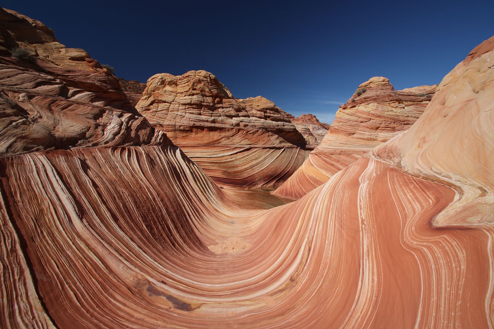
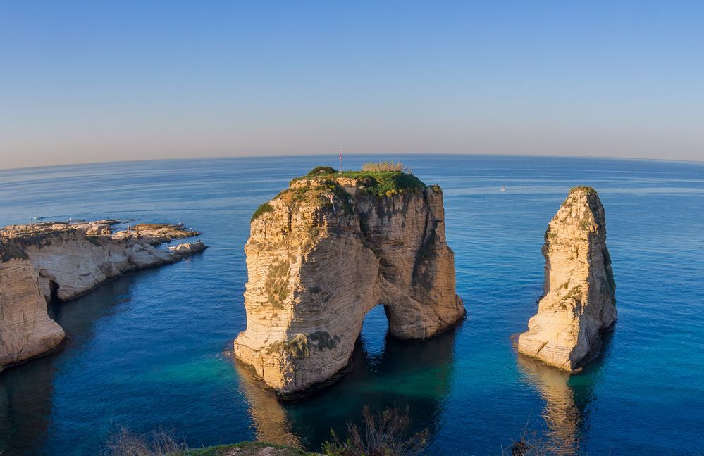
Vermillion rliffs and Raouche rocks
In our case, we'll be more interested in hydraulic erosion, which generally is the process by which water transforms terrain over time. This is mostly caused by rainfall, but can also be caused by ocean waves hitting the shore or alternatively the flow of rivers.
One resource that helped Sebastian Lague figure out hydraulic erosion for his own attempt was Hans Theobald Beyer's bachelor thesis on this very topic, which describes a particle based approach for the erosion of a height map:
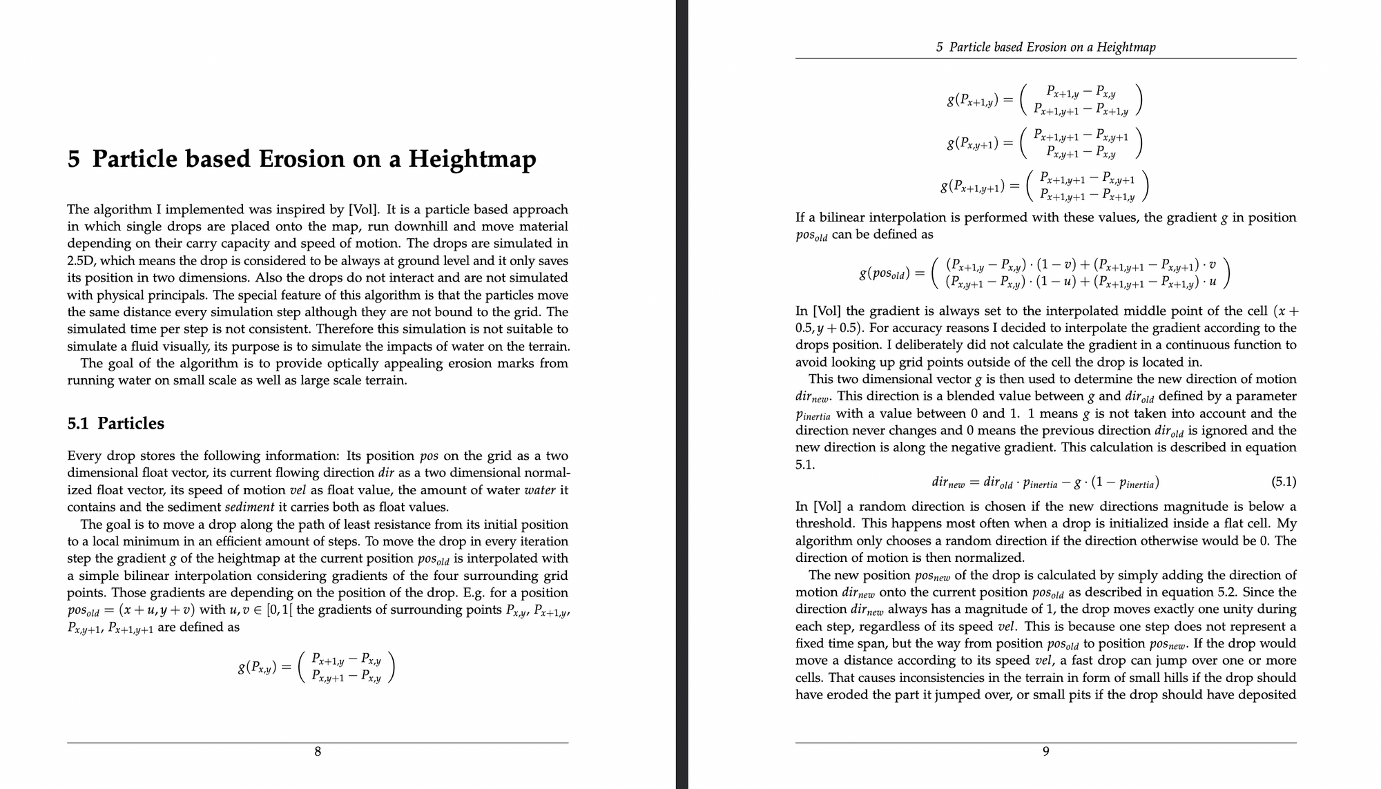
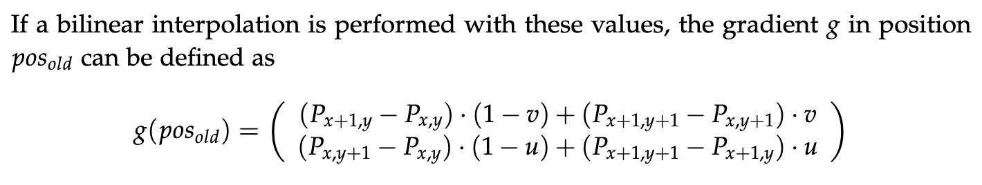
The first paragraph of the fifth chapter gives a good overview of the erosion algorithm. It is summarized as follows:
It is a particle based approach in which single drops are placed onto the map, run downhill and move material depending on their carry capacity and speed of motion. The drops are simulated in 2.5D, which means the drop is considered to be always at ground level and it only saves its position in two dimensions. Also the drops do not interact and are not simulated with physical principals. The special feature of this algorithm is that the particles move the same distance every simulation step although they are not bound to the grid. The simulated time per step is not consistent. Therefore this simulation is not suitable to simulate a fluid visually, its purpose is to simulate the impacts of water on the terrain.
He adds:
The goal of the algorithm is to provide optically appealing erosion marks from running water on small scale as well as large scale terrain.
The technical paper is actually very approachable and every step is clearly explained, so I recommend reading it for yourself if you are interested in learning more. But otherwise here's a brief explanation of how Nat's simulation works. The entire simulation can be done in a large nested loop, where the outer loop iterates over the number of rain drops we want to simulate, and the inner one simulates how long we want the trajectory/path of the raindrop to be:
for (let j = 0; j < nDrops; j++) {
  // stuff here
  for (let i = 0; i < maxIterations; ++i) {
    // stuff here
    // there are a bunch of stopping conditions here
  }
}
After choosing a random position on the heightmap, where we want the raindrop to land, we're gonna want to simulate it traversing and rolling down the heightMap. These raindrops are then going to carve out shapely ridges and deposit sediment at the bottom of valleys. A good visualiztion for what this looks like over the course of the simulation can be seen in Job Talle's write up on the same algo:
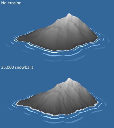
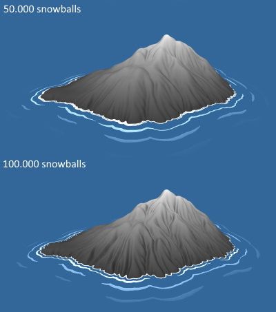
Job calls the raindrops 'snowballs' instead.
To figure out where the raindrop needs to go, we first need to compute the gradient at the current position of the raindrop. The gradient here, is a vector pointing in the direction of 'least resistance', meaning that in most cases the raindrop will be rolling downwards, and maybe sometimes a little upwards if it reaches a valley and has some momentum. For this purpose Nat devised a separate function called calculateHeightAndGradient(mp, posX, posY) that takes in the current position of the drop as well as the height map:
function calculateHeightAndGradient(mp, posX, posY) {

	// flooring the coordinates to use them as grid indices
    let coordX = floor(posX);
    let coordY = floor(posY);

	// the fractional part stored separately
    let x = posX - coordX;
    let y = posY - coordY;

	// values of the surrounding grid entries
    let heightNW = mp[coordX][coordY];
    let heightNE = mp[coordX + 1][coordY];
    let heightSW = mp[coordX][coordY + 1];
    let heightSE = mp[coordX + 1][coordY + 1];

	// bilinear interpolation
    let gradientX = (heightNE - heightNW) * (1 - y) + (heightSE - heightSW) * y;
    let gradientY = (heightSW - heightNW) * (1 - x) + (heightSE - heightNE) * x;

    let ht =
        heightNW * (1 - x) * (1 - y) +
        heightNE * x * (1 - y) +
        heightSW * (1 - x) * y +
        heightSE * x * y;

    return [gradientX, gradientY, ht];
}
What's happening here? Firstly, because the raindrops don't always exactly land on the grid and can have a fractional part in their coordinate values, we'll want to remove this fractional part and store it separately. This can be done by simply flooring the coordinate values and then subtracting them from the original value again. We need the floored values to access the height map array and get the four grid entries that surround our raindrop. We need the elevation value of these entries to estimate the gradient.
This is done with a formula called bilinear interpolation, and essentially takes into consideration where the raindrop falls in between the grid entries. If it is closer to the top-left cell for example, then the values of that cell are weighted more heavily against the values of the other 3 cells. Here the same is done for the height value as well.
Additionally, the direction of the raindrop is computed as a combination of the old direction and this newly computed one, by interpolating them with an inertia parameter. Nat fixed this parameter to 0.5.
Now that we have a way to simulate the raindrop traversing the height map we still need to make it pick up and transport material in form of sediment, as well as define conditions for when to drop it off, such that it spreads it across the height map as it traverses it. This part of the procedure is a bit complicated and there's rather a lot of variables that need to be kept track of, but I'll try to keep it simple and not get lost in the details. The heart piece of the nested loop is the condition that determines if new sediment needs to be picked up, or alternatively if some amount of sediment needs to be dropped off:
if (sediment > sedimentCapacity || deltaHeight > 0) {
	// deposit
else{
	// erode
}
Here the variable sediment is how much material the current raindrop is holding, whereas the variable sedimentCapacity represents how much material the drop can contain at any given moment, it is calculated as a function of several other factors:
let sedimentCapacity = max(-deltaHeight * speed * water * sedimentCapacityFactor,minSedimentCapacity);
These factors being the drop's speed, how much water it still holds as well as how much distance it has traversed (difference between current height and previous height). The second clause in the condition simply triggers when the drop rolls upwards, which can determined by a positive change in height. As for the deposition code, we need to calculate how much of the carried sediment needs to be deposited:
let amountToDeposit = deltaHeight > 0 ? min(deltaHeight, sediment)
: (sediment - sedimentCapacity) * depositSpeed * depositMap[_nodeX][_nodeY];
sediment -= amountToDeposit;
The calculation differs based on the condition that triggered the deposition. If we're rolling upwards, we deposit an amount equal to how much we traveled upwards, or the entire sediment that is currently held if the distance is greater than that amount. Otherwise, if the deposition is triggered by a sediment amount exceeding the capacity, we drop off an amount that is a function of the deposition speed and the entry in the deposition map that we created earlier (while creating the height map). This value is set to 0.001 and basically scales the sediment amount that is dropped off. This amount is then distributed to the four neighbouring cells again with bilinear interpolation.
In the case of erosion, we don't actually only pick up sediment from the four neighbouring cells, but rather from all cells within a given radius. How much sediment is taken is based on an influence parameter:
let influence = 1.0 / sq(dropRadius + 1);
let amountToErode = min((sedimentCapacity - sediment) * erodeSpeed, -deltaHeight) * erodeMap[_nodeX][_nodeY] * influence;
Again, here the amount to erode is either the distance that is traversed or the remaining capacity scaled by the speed (if that is less than the distance traversed), multiplied by the erodeMap parameter which is set to 0.1 as well as the influence parameter that depends on the size of the erosion radius.
And I believe this is the gist of the erosion algorithm, I tried to simplify everything as much as possible. There is still many more parameters that take part in the overall procedure; I could probably play and break the code for hours on end. Maybe I will do a separate article on this hydraulic erosion algorithm in the future and attempt to break it down in more detail.
Pre-computing the Scribbles
So let's backtrack a little bit. We've explored the prepareHeightMap() and the erosion() functions, and have acquired a general understanding of how they work. Now let's jump back to the setup() function where we left off, and see how the eroded height map is used to position the colorful scribbles that make up the graphics.
Directly after having prepared the height map, we can see another group of variables being declared:
// number of scribbly strokes to be drawn
let nShapes = 8000;

// number of trees and bushes
let nCircles = nShapes * 0.2;

// threshold condition for drawing the plants/trees/bushes
let treeToScrubThresh = random(0.18, 0.28);
let plantThresh = constrain(random(0.3, 0.5), 0.3, 0.45);
let plantSide = random([-1, 1]);
let plantSlopeLeniency = random(0.01, 0.1);
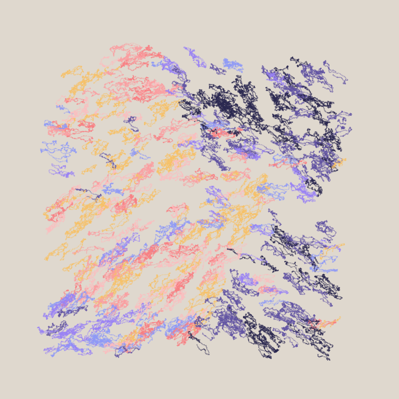
These are quite important as they represent the number of scribbly strokes as well as the amount of scribbly vegetation that will be drawn to the canvas. Zeroing either one of the parameters has the following effect:
nShapes=0 | nCircles = 0 respectively
Additionally, a couple of parameters represent thresholds that control the placement of the vegetation. Now there's actually a bunch of loops, each one being responsible for a particular type of item in the scene. We'll first have a loop at the second one which allocates the scribbly strokes that make up the terrain. Also keep in mind that right now we're just creating the objects and not actually drawing them yet to the canvas. Inside of this loop we have:
// pick a random coordinate to draw a scribble
let x = random(targetSz);
let y = random(targetSz);
let z = y + 10; // z index required to sort for the top down drawing order

// floor and constrain the picked coordinate to get the corresponding height map entry at that point
let i = constrain(floor(map(x, 0, targetSz, mapTrim, mapW - 1 - mapTrim)), 0, mapW - 1);
let j = constrain(floor(map(y, 0, targetSz, mapTrim, mapH - 1 - mapTrim)), 0, mapH - 1);
let ns = hMap[i][j];
Next we have a couple of interesting lines:
x += cos(ns) * warpSz;
y += sin(ns) * warpSz;
y += map(ns, 0, 2 * TAU, 0, 1) * terrainHt;
These lines add a slight visual swing/waviness to the scribbly field. We can accentuate this more by cranking the warpSz parameter:
warpSz=0 | warpSz=50 | warpSz=200 respectively
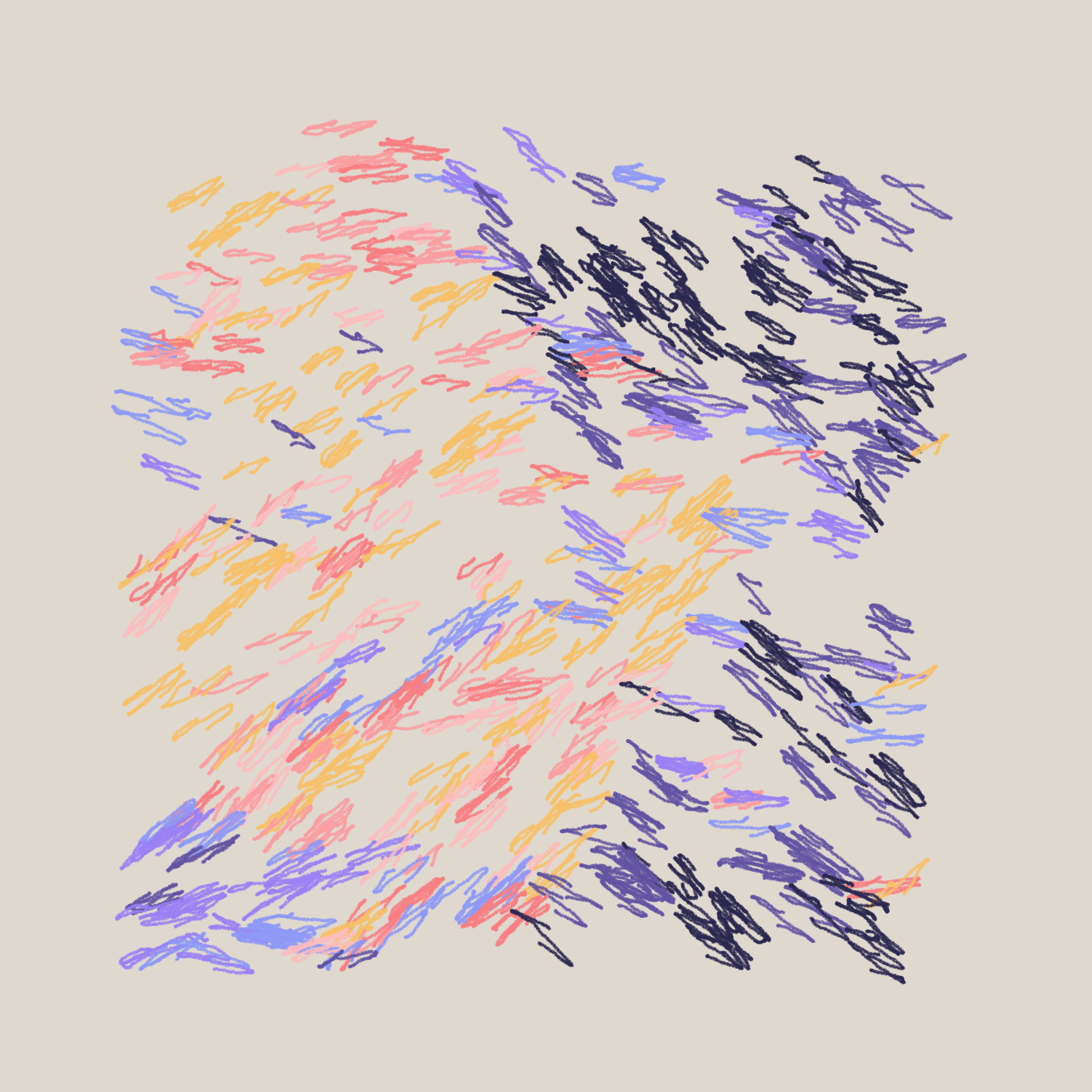
The next line is a rather important one, the best way to show what it does is by zeroing it out:
let nrm = _normalize(hMapNormal(i, j)); // 0
It determines the actual orientation of the scribbles. Let's see what the function hMapNormal() does:
function hMapNormal(i, j) {
  let _i, iDir = 1;
  let _j, jDir = 1;

  return _createV(
    (hMap[_i][j] - hMap[i][j]) * iDir,
    (hMap[i][_j] - hMap[i][j]) * jDir);
}
I'm not 100% certain of this one, but I think I have an idea of what is happening here. I believe that this calculation is called finite differencing and essentially computes the gradient vector at the given coordinates on the height map. The computed gradient vector, in this case, is essentially also a normal vector to the surface. Adding half a rotation, this normal vector is then used to determine the slant of these scribbles.
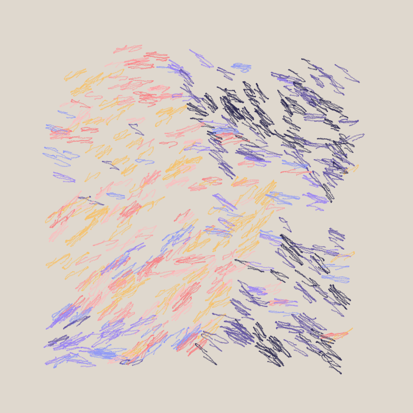
The two parameters minStrokeLength and maxStrokeLength determine how long the drawn scribbles end up being, we can plug in different values here for a different style:
let minStrokeLen = 15;
let maxStrokeLen = 30 * 0.8;

let nScribbles = max(1, floor(map(pow(abs(y - z), 1), 0, pow(abs(terrainHt) + abs(warpSz), 1), 1, random(1, 3))));

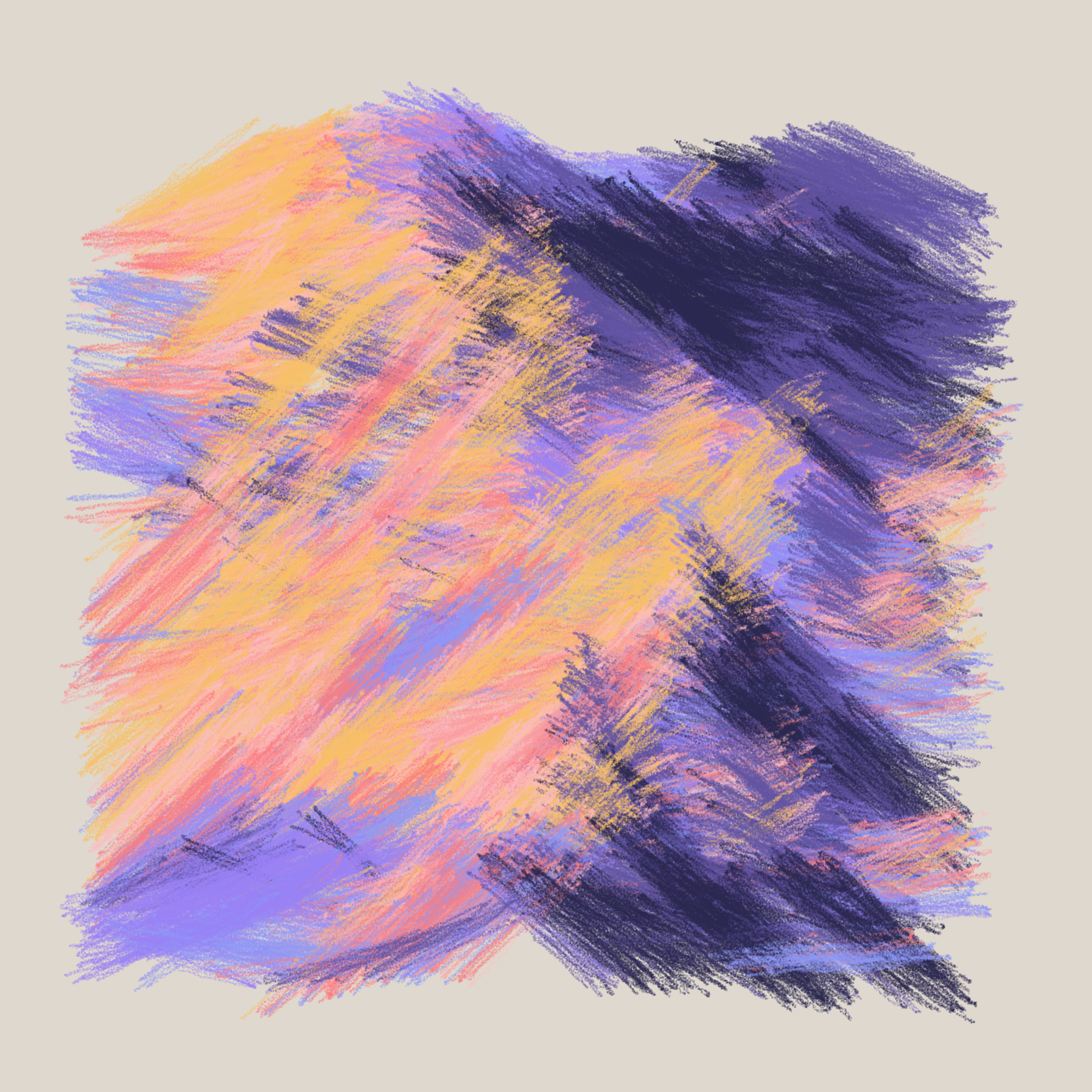
minStrokeLen = 1, maxStrokeLen=10 | minStrokeLen = 5, maxStrokeLen=15 respectively
As for the nScribbles parameter, it determines how many layers of strokes there are within one scribble, hardcoding these values to different numbers we obtain different aesthetics:
nScribbles=1 | nScribbles = 10 respectively
The variable nScribbles is then used as an upper bound for the iterations of another loop in which we will actually create the different scribble objects and store them:
for (let k = 0; k < nScribbles; k++) {
    let r = constrain(
    	map(nrm2, 0.0001, 0.0008, maxStrokeLen, minStrokeLen),
    	minStrokeLen,
    	maxStrokeLen
    );

    let scribble = new SketchyEllipse(
        x, y,
        5, r * random(0.9, 1.1),
        random(1, 2)
    );
}
We can also play a little here and see what aesthetic effect the variable r has on the sketch:
r=1 | r=5 | r=50 respectively
It is essentially the length of the scribbly strokes, and apparently the nrm2 value that was computed earlier determines where the length falls within that range. The nrm2 being another normal vector to the heightmap. The parameter before must then be the width:
w=2 | w=3 | w=50 respectively
Here Nat chose to fix it to a medium value of 5.
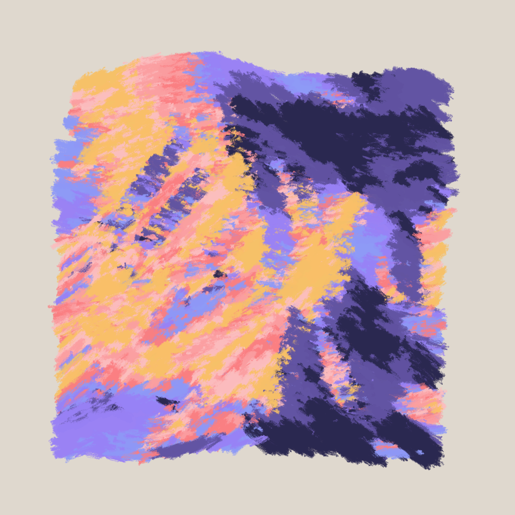
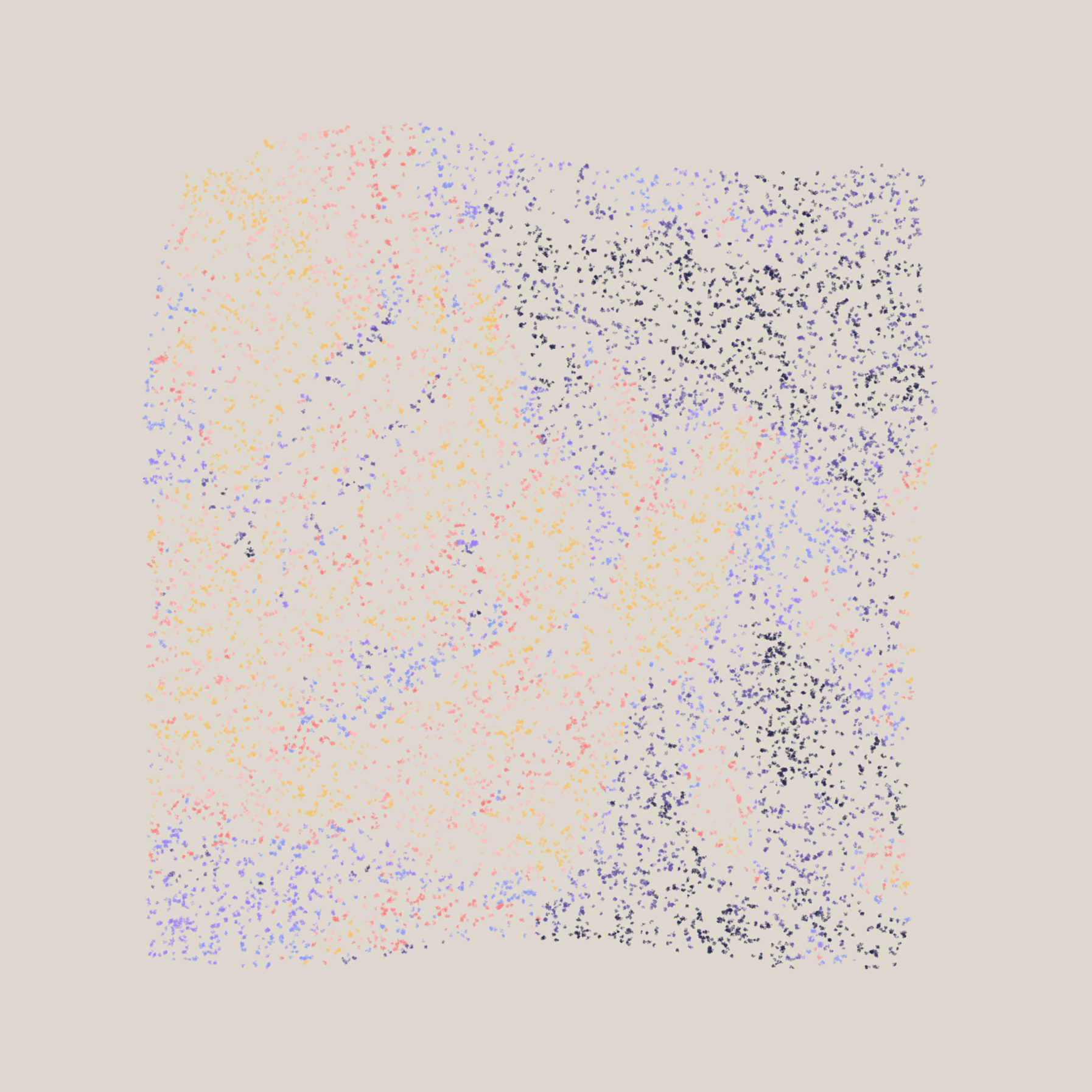
Scribbly Pen Simulation
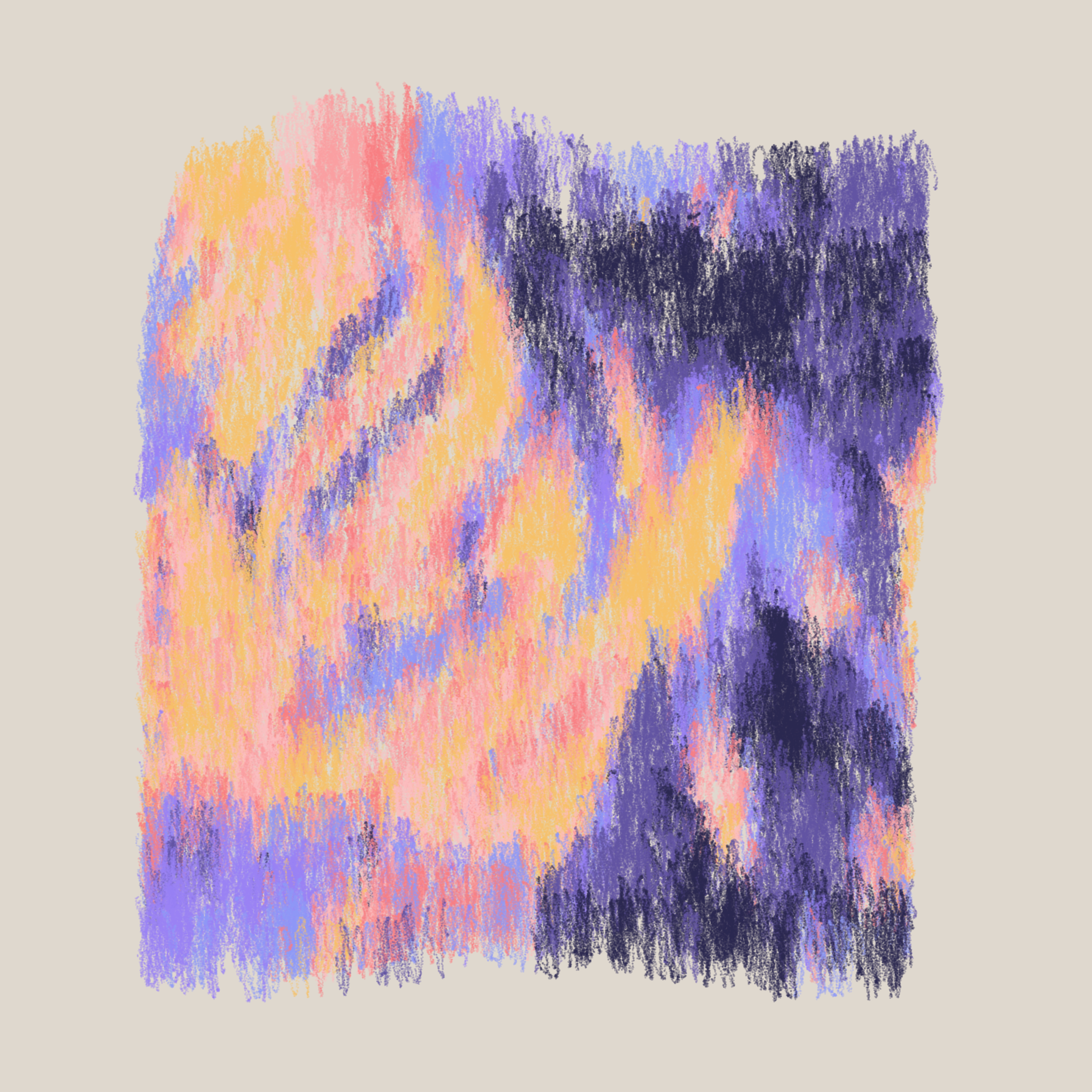
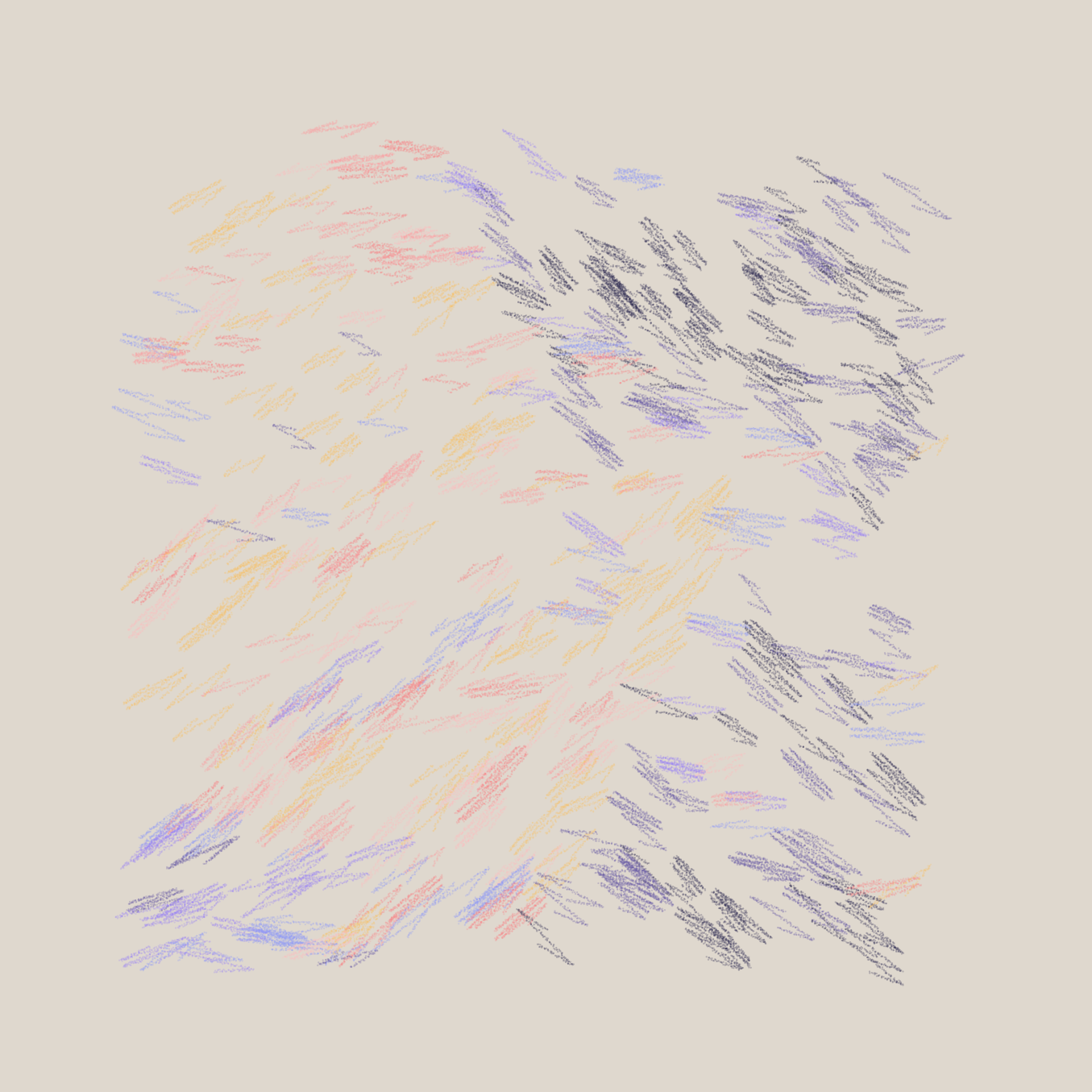
A lot of thought has also gone into how the individual scribbles are composed . Here's the token with a reduced number of scribbles, making it easier to see their individual shape:
I already had a hunch about how the scribbles are drawn. The code confirms it though. The scribbles actually consist of many small points, that are stored within an array called 'points', which also is a member variable of the scribble object. What interests me is getting an insight into how these points are positioned.
A closer look at the sketchyEllipse's constructor reveals the following code:
let nSubSteps = max(2, round(rx / hatchDensity));
for (let i = 0; i < nSubSteps; i++) {
    let x = map(i, 0, nSubSteps - 1, -rx, rx);
    let ht = ry * sqrt(1 - sq(x) / sq(rx))

    this.points.push({x: x, y: ht});
    this.points.push({x: x, y: -ht});
}
However, that's not all there is to it, Nat actually put together a really convincing scribble simulator! This loop creates the points that make up the scribble and stores them in an array, but that doesn't draw them to the canvas just yet. For that we'll have to go and have a look at the sketchyShape() class.
The object oriented paradigm is used for the code that handles the different scribbles: the SketchyEllipse() class - that was used to create the terrain scribbles - extends another class and inherits functionality from it:
class SketchyEllipse extends SketchyShape {
    constructor(cx, cy, rx, ry, hatchDensity, outline) {
        super();
        //other stuff
    }
}
In the SketchyShape class we can find the code that makes use of the precomputed points array to actually draw the scribble. The way that this works is really cool, we actually simulate a pen tracing these points rather than just drawing the points densely close to each other.
The pen in this manner, is represented by a vector: initially positioned at the first point in the array, we iteratively nudge this pen in the direction of the following point:
let targetPoint = this.points[this.penTargetIndex];
let dx = targetPoint.x - this.pen.x;
let dy = targetPoint.y - this.pen.y;
let ax = dx * this.acc;
let ay = dy * this.acc;
this.penV.x += ax;
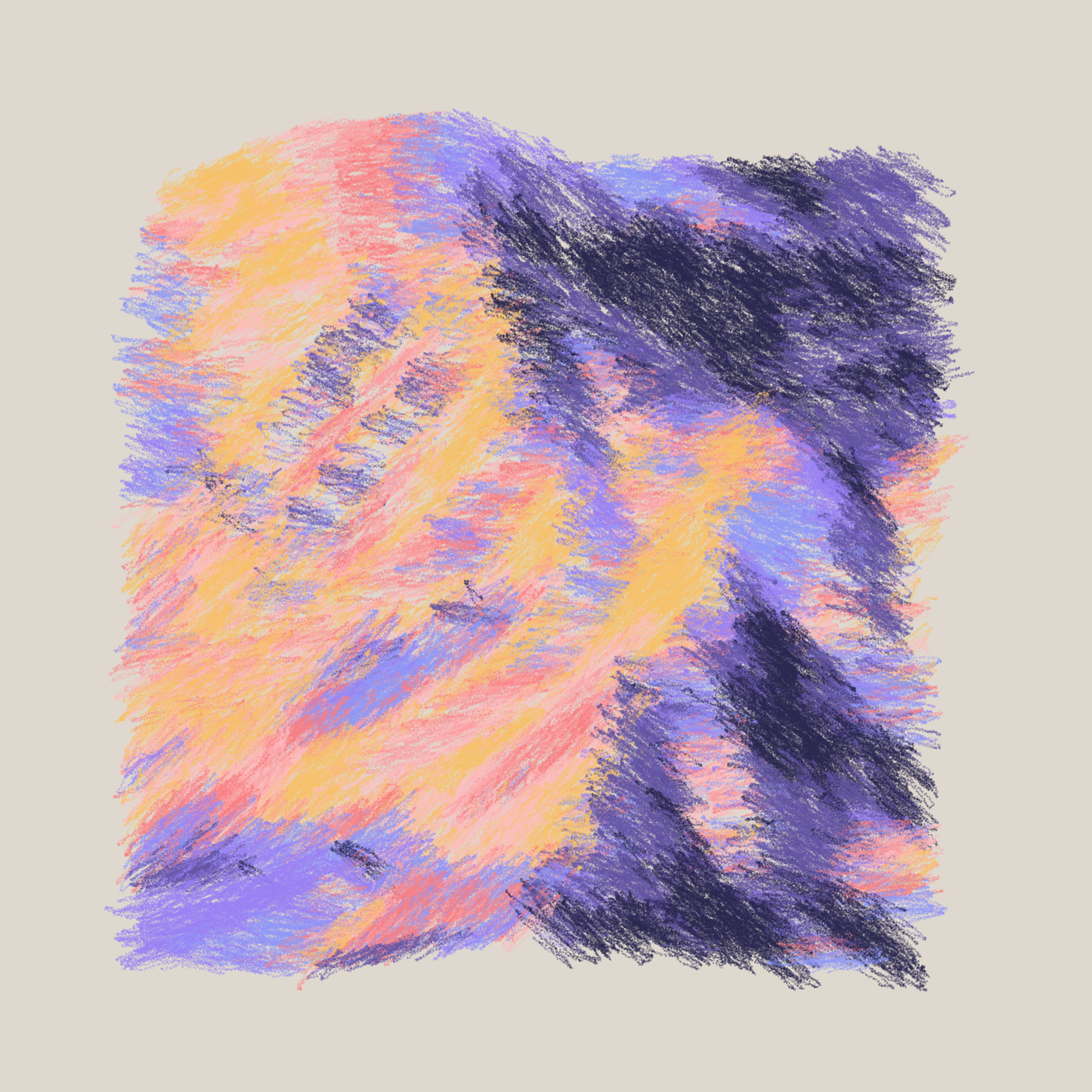
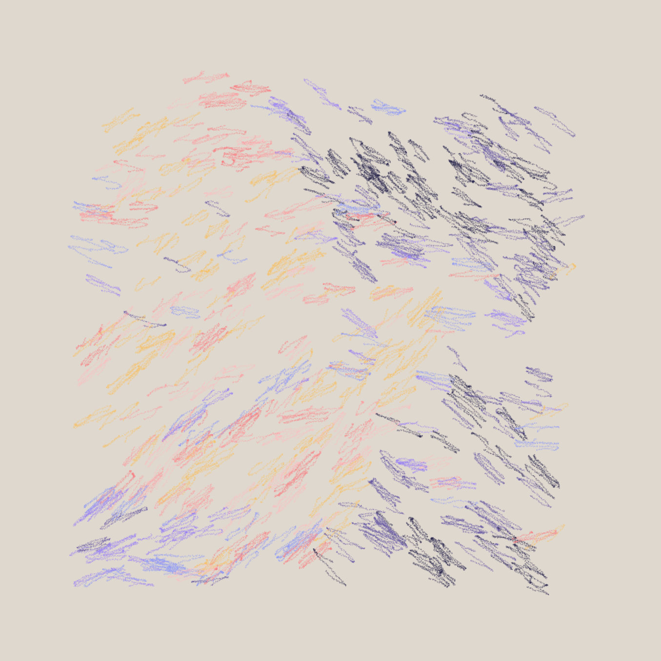
this.penV.y += ay;What's cool here is how we move the pen in the direction of the next point. Instead of doing it in a linear manner, there's an accuracy parameter that controls how accurately we are nudging the pen in the direction. Changing this parameter we can get some interesting variations:
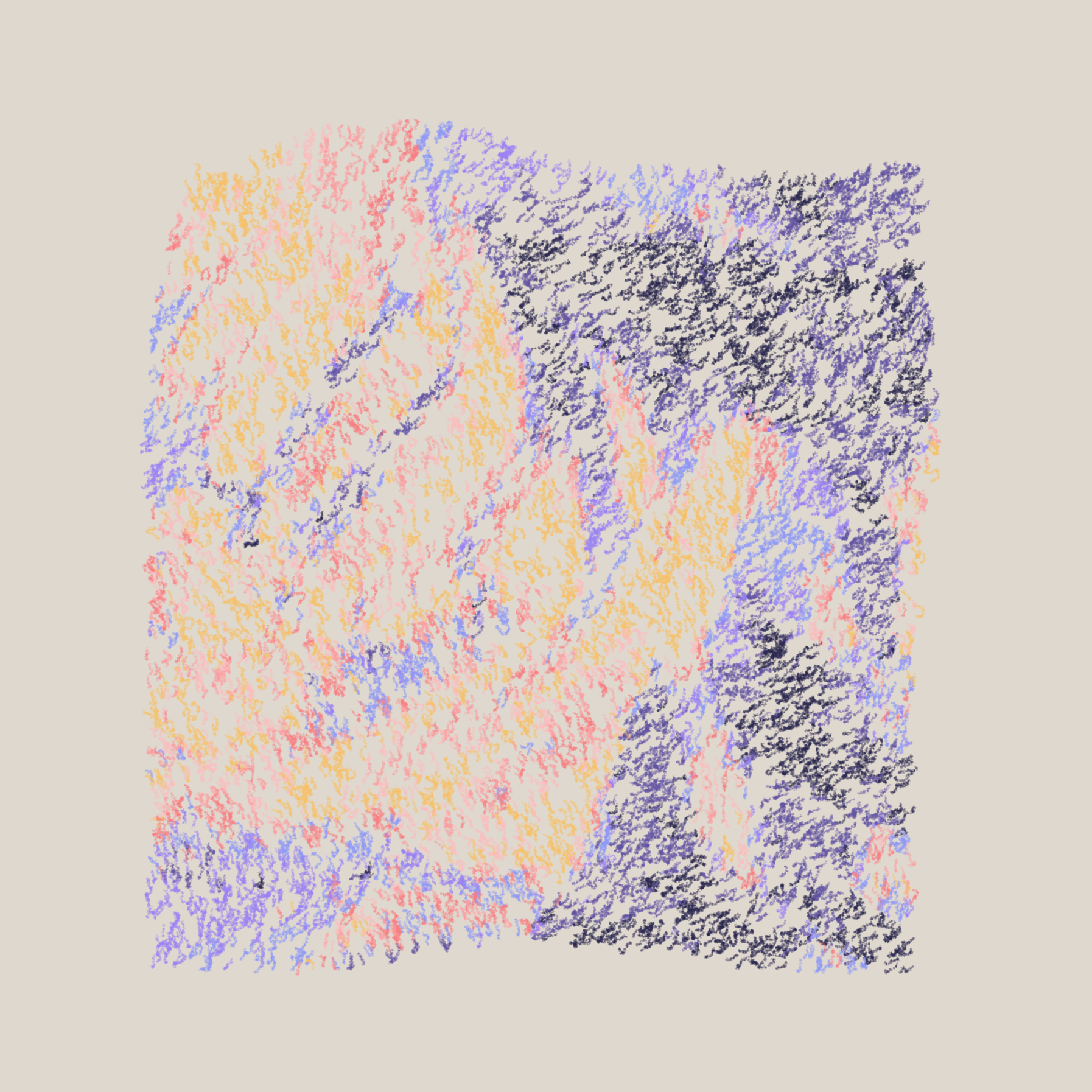
this.acc = 2 | this.acc = 0.004 | this.acc = 0.001 respectively
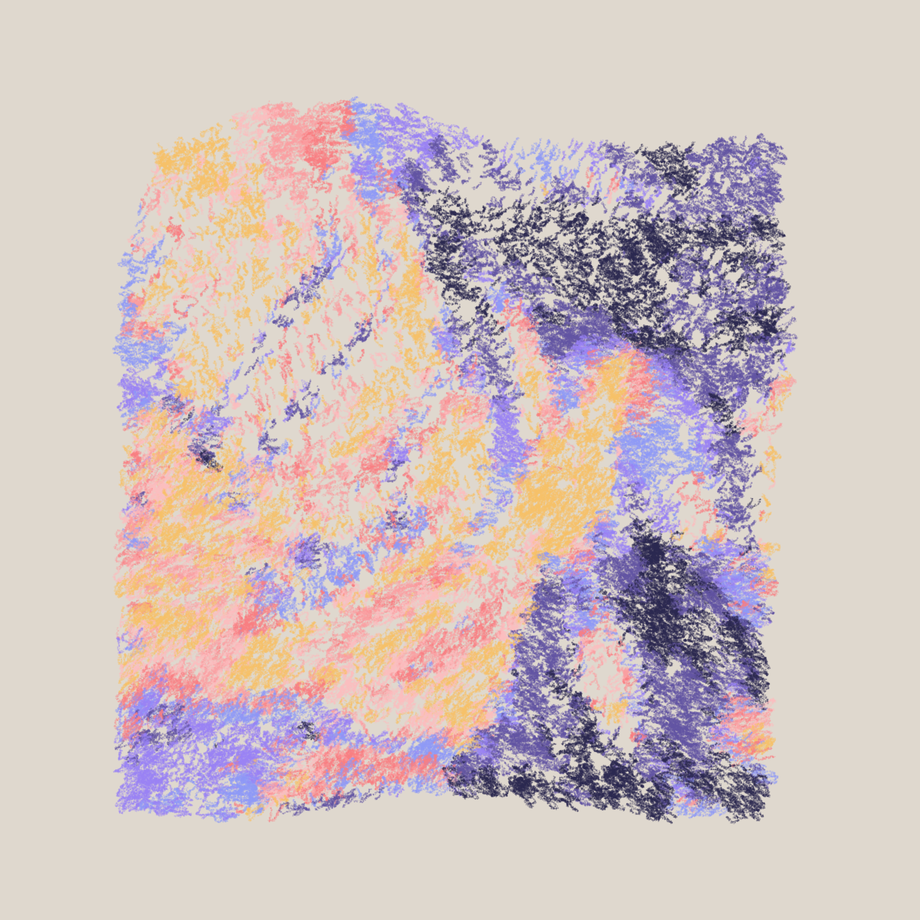
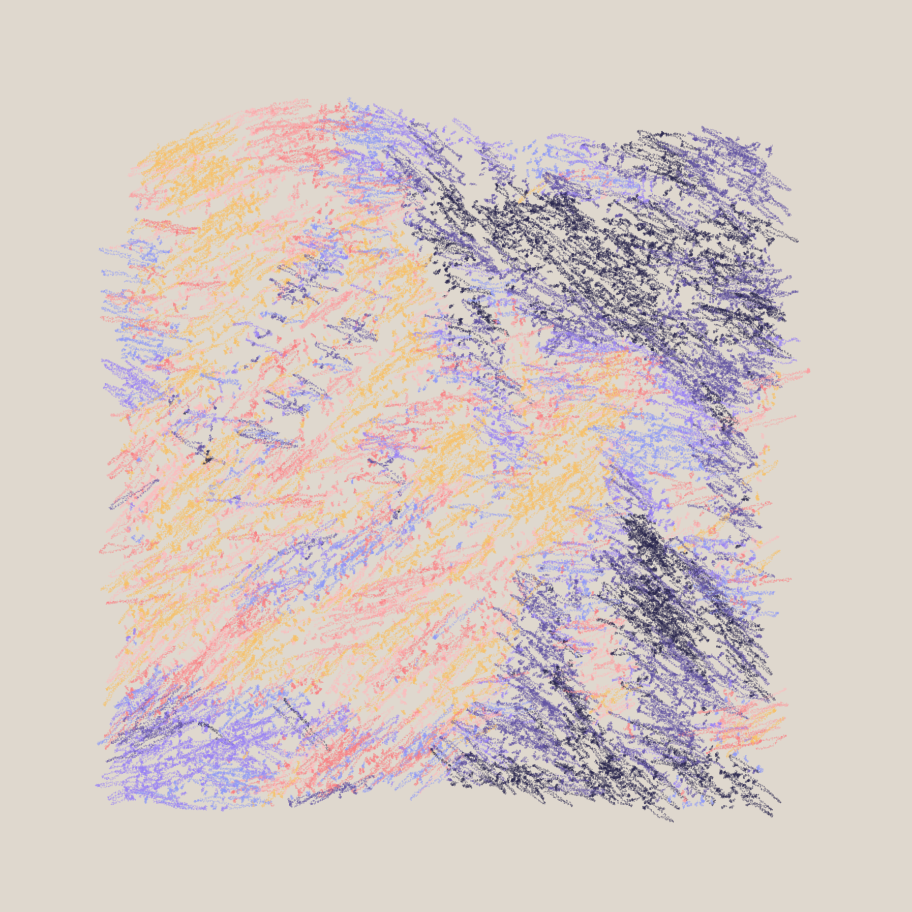
There's a bunch of other parameters that control the behaviour of the pen, one of them being a density parameter, that determines how many points are drawn when we nudge the pen forward (the pen doesn't draw lines, but rather many points in between the path points):

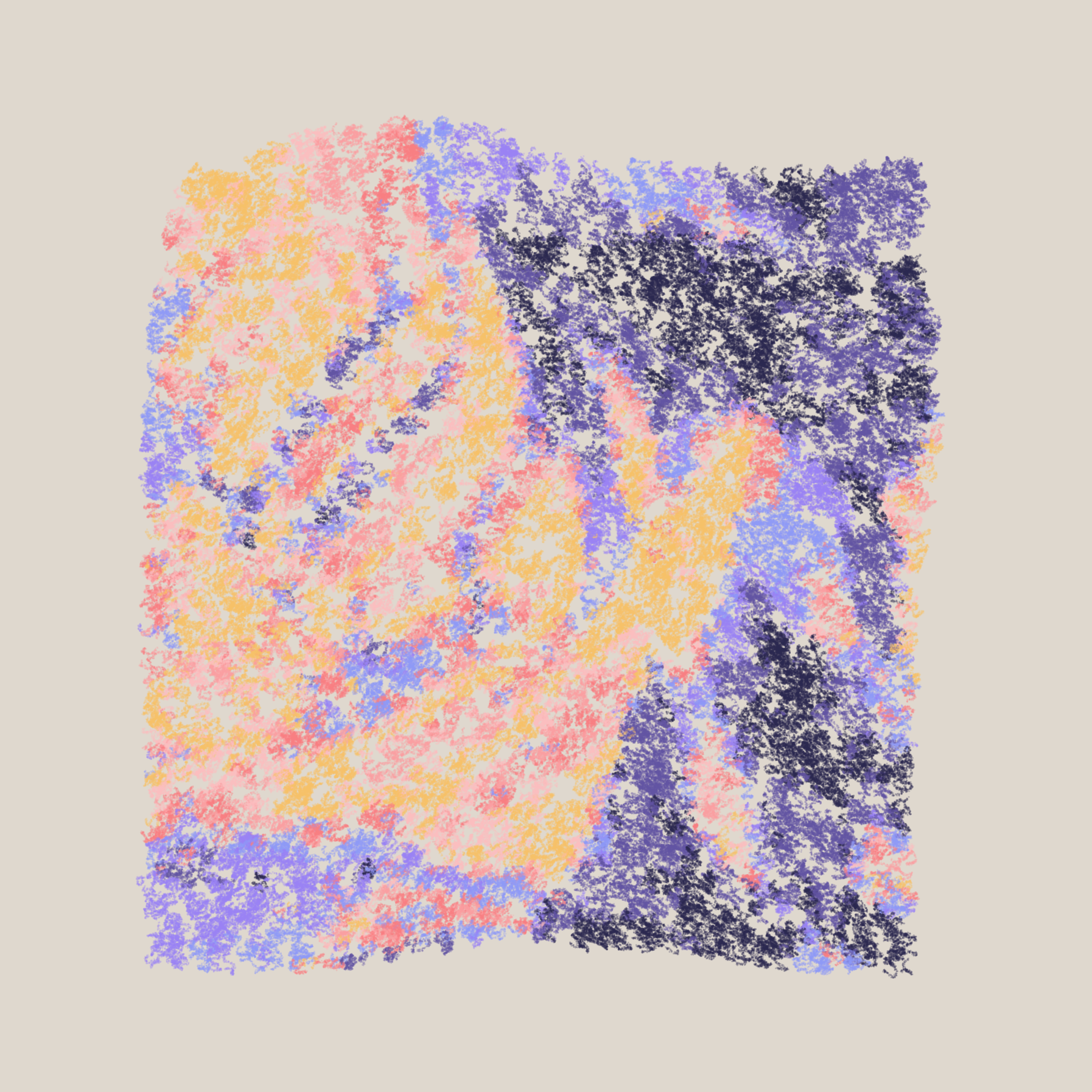
density = .01 | density = 5 | density = 15 respectively
Overall, this is an incredibly genius way to go about drawing the scribbly strokes, and it shows how much care went into the details. The other shapes in the scene, the trees for example, use this same strategy; a number of other classes also inherit from the SketchyShape class, but are setup with slightly different parameters.
Light Map and Colours
One last thing to address here is the colour selection mechanism, how it ties into the light map and how it creates such beautiful shadings of the terrain. Let's exiting the shape drawing classes, and find ourselves back inside of the setup function where we're precomputing the scribbles. We can see that the colours of the scribbles are selected based on the corresponding value in the light map at a given position:
let dt = lMap[i][j];
let lightValue = norm(dt, -1, 1);
let c = paletteColor(lerp(landValue, lightValue, abs(lightValue - 0.5) * 2));
scribble.setColor(color(red(c),green(c),blue(c),64)); // slightly transparent colors
We used the light map value to find the index of a specific color in the palette array. How is this light map computed? We have to visit the map.js script file one final time for this:
function prepareLigthMap() {
    for (let i = 0; i < mapW; i++) {
        let row = [];
        for (let j = 0; j < mapH; j++) {
            let nrm = _normalize(hMapNormal(i, j));
            let dt = _dot(nrm, lgt);
            row.push(dt);
        }
        lMap.push(row);
    }
}
It seems we're computing a dot product of some sort. At the very beginning of the sketch we've declared a variable that represents the angle of the light source:
lightAngle = -PI / 2 + (random(1) < 0.5 ? -1 : 1) * PI / 3;
lgt = _normalize(_createV(cos(lightAngle), sin(lightAngle), 0));
This angle is necessary to compute the light map. The values of the light map are essentially the dot product between the surface normals of the height map and the angle of this light source.
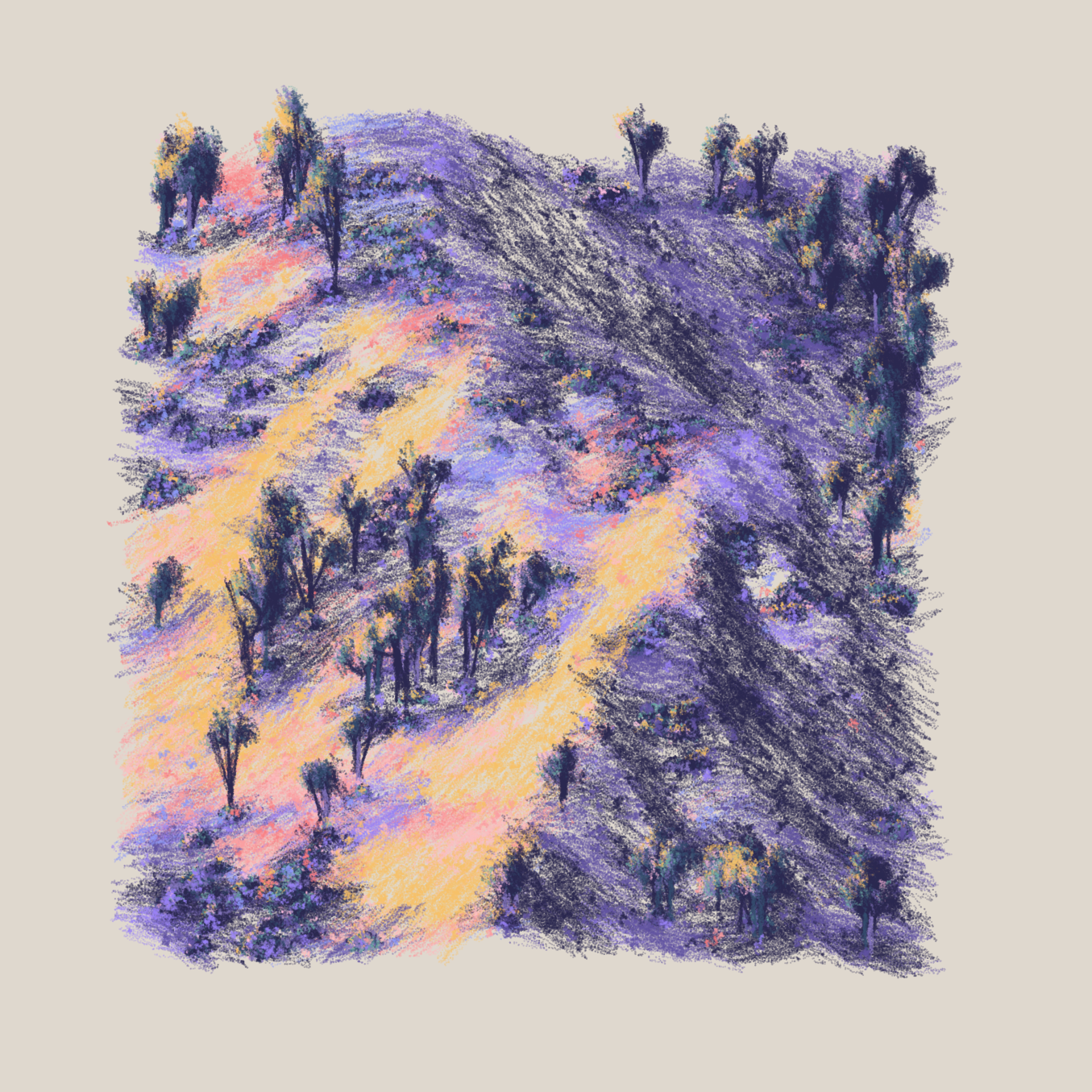
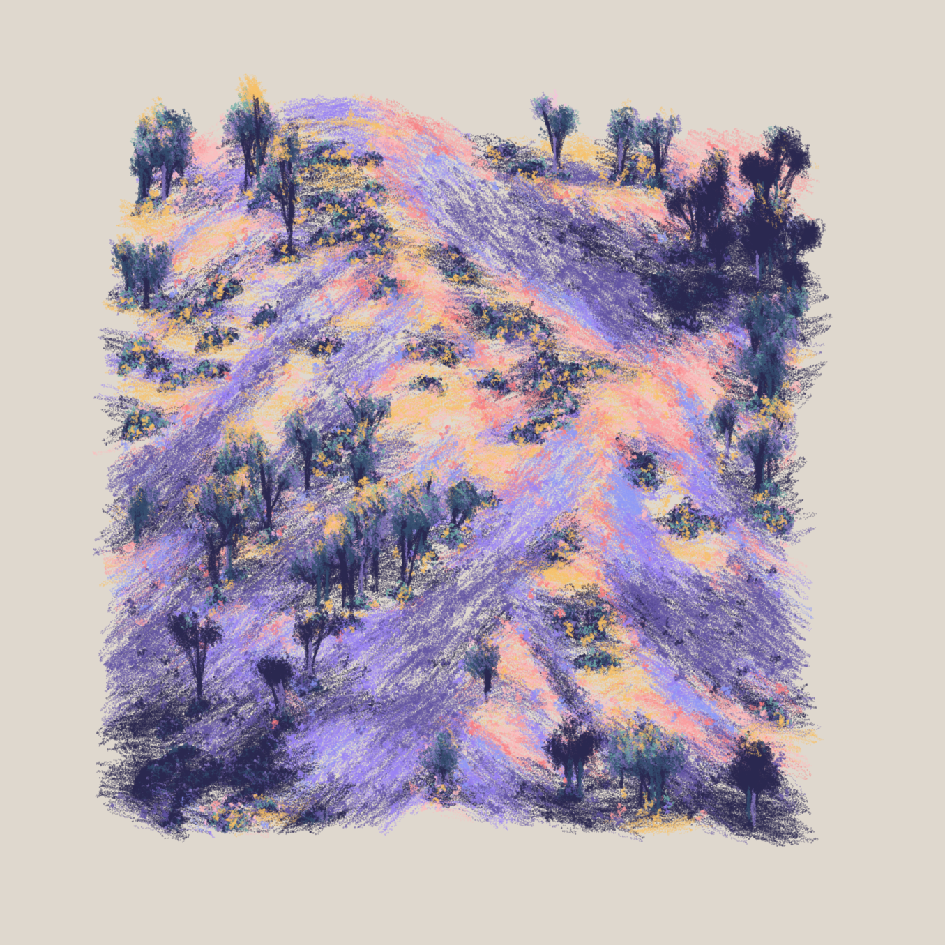
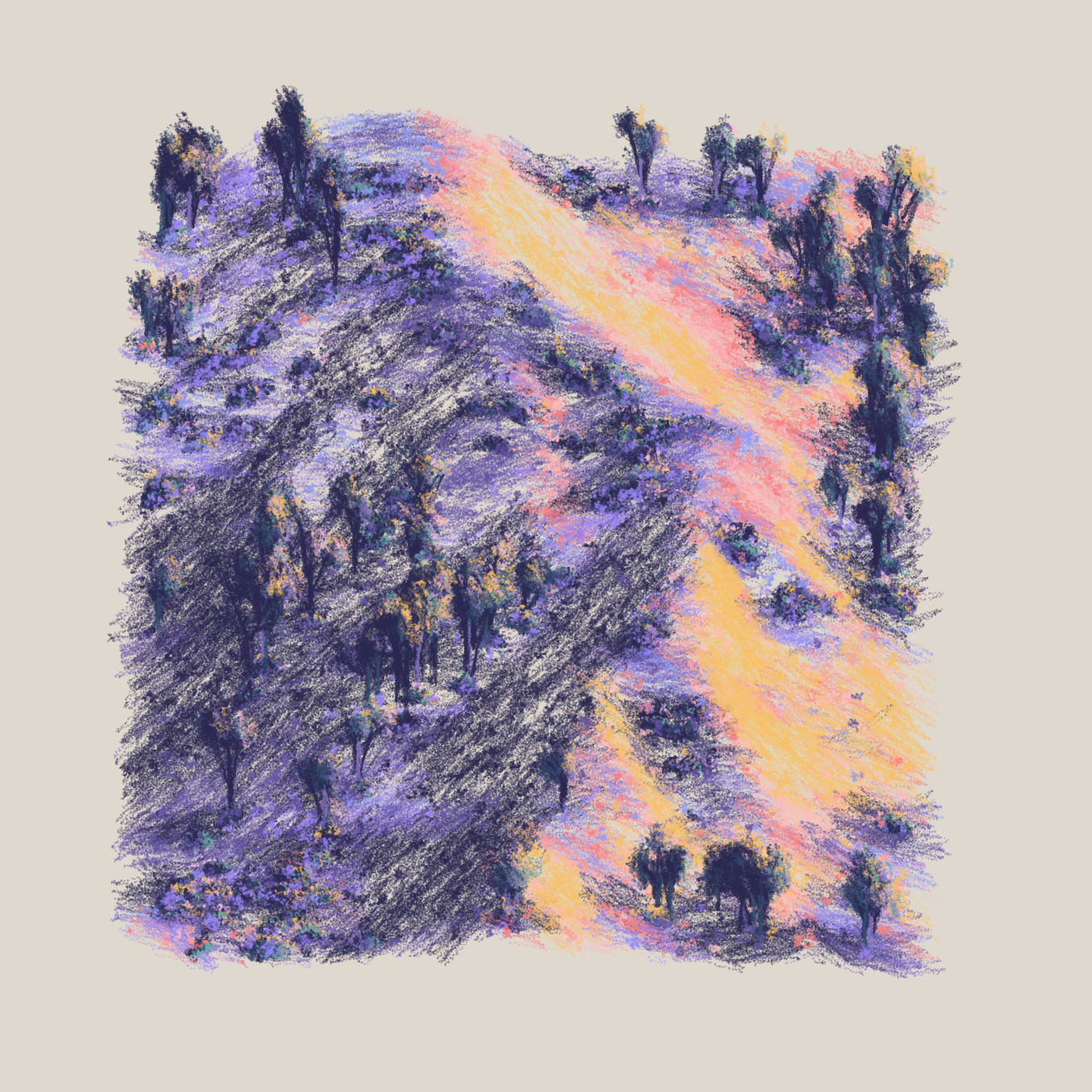
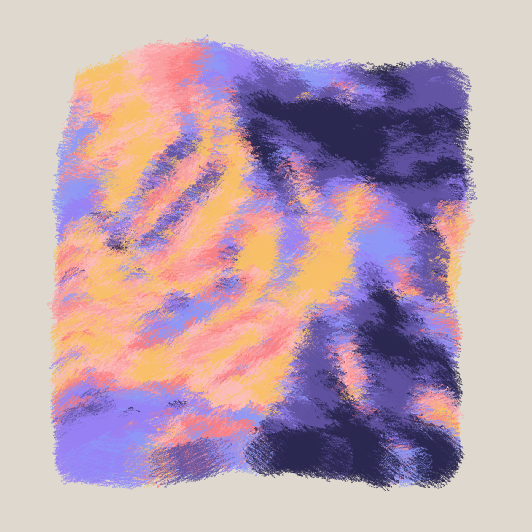
Angle of the light source at 0, -PI/2 and -PI respectively. Insane right?
With the seed fixed, we can change the angle of this light source, almost making it seem as if we're viewing the scene at different times of the day.
The question is, why do we need to compute the dot product?
The vector dot product (or inner product) of the normalized vectors N and L is a measure of the angle between the two vectors. The smaller the angle between the vectors, the greater the dot-product value will be, and the more incident light the surface will receive. | The Cg Tutorial
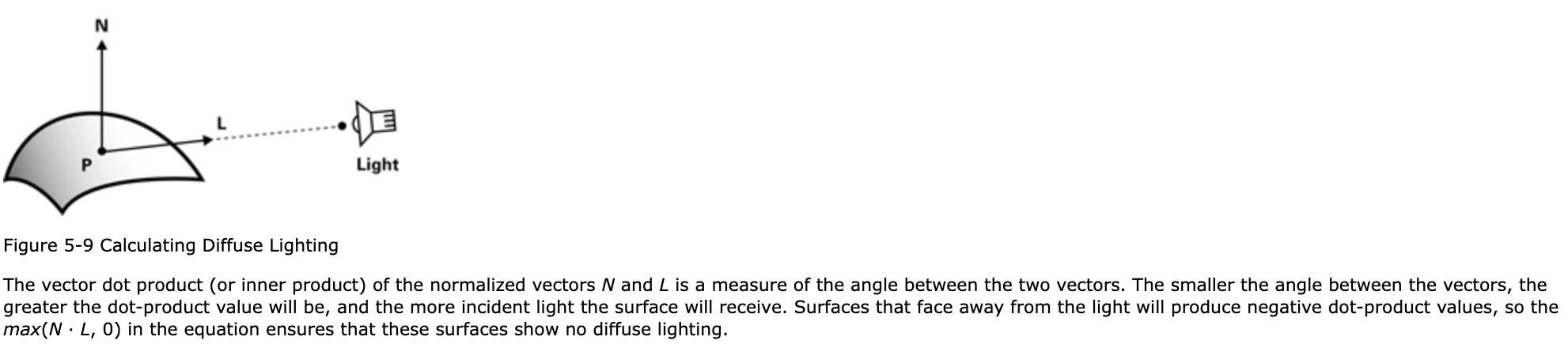
The dot product is required how large the angle between the light source and the surface normal at a specific point on the height map. Using this dot product to select the colors then makes it so that steeper surfaces angled towards the light source are assigned brighter colors, whereas surfaces not facing the light surface are assigned darker colors.
Closing Thoughts
Nat's piece isn't just visually stunning, it also is an amazing feat of generative art. It was a genuine joy to dig through the code and figure out how the different components work together. I hope this breakdown is as much an inspiration to you as Nat's code was to me.
Big shoutout to Nat, go show him some love on social media and check out his other tokens on fxhash! Yes, he's got more amazing stuff!
Hope you enjoyed reading this! What project would you like me to tackle next? Leave me suggestions in the comments below or over on Twitter. Lastly, consider signing up to the mailing list to get updates whenever there's new content, as well as sharing this article with a friend (it helps out a lot)! - Otherwise, happy sketching! Cheers!